Compare groups
Statistical comparison
Very often we need to compare two groups of users using some metrics. It can be during A/B test results analysis, or comparing two user segments from different channels, or comparing cohorts of users and etc.
Basic example
This notebook can be found here
or open directly in google colab.
In this tutorial we will use a simple dataset of user activity logs in app or web-site during hypothetical A/B test. It has raw behavior event-level logs as well as additional information, specifying the particular user in the test or control and some transaction information.
We start from importing retentioneering and sample datasets:
import retentioneering

# load sample data
data = retentioneering.datasets.load_simple_ab_test()

data.head()
| user_id | event | timestamp | user_backet | transaction_value | transaction_ID | |
|---|---|---|---|---|---|---|
| 0 | 219483890 | catalog | 2019-11-01 17:59:13.273932 | test | NaN | None |
| 1 | 219483890 | product | 2019-11-01 17:59:28.459271 | test | NaN | None |
| 2 | 219483890 | cart | 2019-11-01 17:59:29.502214 | test | NaN | None |
| 3 | 219483890 | catalog | 2019-11-01 17:59:32.557029 | test | NaN | None |
| 4 | 964964743 | catalog | 2019-11-01 21:38:19.283663 | test | NaN | None |
We can see regular columns with information about user actions (‘user_id’, ‘event’, ‘timestamp’) as well as column regarding A/B test: ‘user_backet’, and columns with transactions information (events ‘payment_done’): ‘transaction_value’ and ‘transaction_ID’.
Next, as usually we need to update retentioneering.config to specify column names for events, user_ids and time:
retentioneering.config.update({
    'user_col': 'user_id',
    'event_col':'event',
    'event_time_col':'timestamp',
})
Let’s explore column ‘user_backet’:
(data
 .drop_duplicates(subset=['user_id'])['user_backet']
 .value_counts())
not_in_test    2624
control         573
test            554
Name: user_backet, dtype: int64
We can see that our dataset has 554 and 573 unique users in test and control groups, correspondingly. Let’s put those user_id’s in separate variables ‘test’ and ‘control’:
test = data[data['user_backet']=='test']['user_id'].unique()
control = data[data['user_backet']=='control']['user_id'].unique()
Now everything is ready to start comparing these two groups using rete.compare() function.
Let’s say we would like to compare conversion rate in the test vs control groups. For this we would need to specify a function that given one user trajectory (in form of dataframe) will return a numerical value, 1 (converted) or 0 (not converted) in our case. Importantly, function must take as an argument a dataframe of one user trajectory, perform any type of calculation and return a single numerical value.
In our case user is considered converted is they have ‘payment_done’ event, so the function definition is very straightforward:
conversion = lambda x: int(['payment_done'] in x['event'].unique())

data.rete.compare(groups=(test, control),
                  function=conversion,
                  test='mannwhitneyu',
                  group_names=('test','control'))
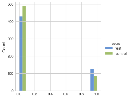
group_1 (mean ± SD): 0.227 ± 0.419, n = 554
group_2 (mean ± SD): 0.148 ± 0.355, n = 573
'group_1' is greater than 'group_2' with P-value: 0.00034
power of the test: 96.15%

- Parameters for function rete.compare():
groups: tuple (g1, g2), where g1 and g2 are collections of user_id`s (list, tuple or set) of two groups for comparison.
function(x): function that takes a single user dataset as an argument and returns a single numerical value (see below for more examples).
test: {‘mannwhitneyu’, ‘ttest’, ‘ks_2samp’}, selected statistical test to test the null hypothesis that 2 independent samples are drawn from the same distribution. One-sided tests are used, meaning that distributions are compared for ‘less’ or ‘greater’. Rule of thumb is: for discrete variables (like conversions, number of purchases) use Mann-Whitney test (‘mannwhitneyu’) or t-test (‘ttest’). For continuous variables (like average_check) use Kolmogorov-Smirnov test (‘ks_2samp’).
group_names - optional parameter to set group names for the output.
alpha - Selected level of significance, to calculate power of the test: probability to correctly reject a H0 when H1 is true. Default value is 0.05.
We can see that in the example above the test group has statistically significantly higher conversion rate than the control group (given P-value threshold for significance 0.05), therefore change must be implemented. Histogram just illustrates how the selected metric is distributed between groups (in the example above metrics can only be 0 or 1).
To illustrate better how to define custom metrics and pass it as an argument to rete.compare() function let’s compare a couple more metrics. Suppose we would like to compare the average check between test and control groups. Again, it’s very easy:
average_check = lambda x: x['transaction_value'].mean()

data.rete.compare(groups=(test, control),
                  function=average_check,
                  test='ks_2samp',
                  group_names=('test','control'))
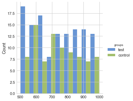
test (mean ± SD): 736.026 ± 149.001, n = 126
control (mean ± SD): 732.980 ± 139.960, n = 85
'test' is less than 'control' with P-value: 0.55199
power of the test: 3.65%

In this case we can see that there is no statistically significant difference in average checks between two groups (P-value is 0.55, selected threshold is 0.05). Note that for continuous variables like average check we used Kolmogorov-Smirnov test. While we can conclude that users in the test group converted to purchase more often than in the control group, there was no effect on the average check.
More complex metrics
Just to illustrate that metrics function can be any complex, let’s consider another example. Suppose we have a separate file, which has all transaction_id’s and their statuses (for example, whether a transaction was already confirmed by the bank or not).
For the demonstration purpose let’s just create such dataframe with randomized data:
import pandas as pd
import random

all_ids = data['transaction_ID'].dropna().unique()
status = pd.DataFrame({'transaction_ID': all_ids,
                       'confirmed': [random.random() > 0.2
                                     for _ in all_ids]})

status.head()
| transaction_ID | confirmed | |
|---|---|---|
| 0 | 7121884 | True |
| 1 | 9641982 | False |
| 2 | 9826287 | True |
| 3 | 9647603 | True |
| 4 | 8125650 | True |
Now, let’s write metrics function confirmed_purch, which will return 1 if user has confirmed transactions or 0 if has not:
def confirmed_purch(x):

    # get list of transactions for user x
    trans_list = x['transaction_ID'].unique()

    # get all status records for transactions from user x
    trans_status = status[status['transaction_ID'].isin(trans_list)]

    # True / False if user has conf transactions
    has_conf_trans = trans_status['confirmed'].sum() > 0

    # convert bool to int:
    return int(has_conf_trans)
It’s very straightforward. Again, function confirmed_purch() takes a single user trajectory as an argument (as pandas dataframe) and returns a single numerical value. Let’s compare our groups using confirmed_purch metric:
data.rete.compare(groups=(test, control),
                  function=confirmed_purch,
                  test='mannwhitneyu',
                  group_names=('test','control'))
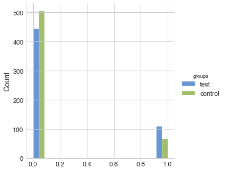
test (mean ± SD): 0.184 ± 0.388, n = 554
control (mean ± SD): 0.122 ± 0.327, n = 573
'test' is greater than 'control' with P-value: 0.00193
power of the test: 85.25%

As we can see, a statistically significant difference in the conversion to confirmed purchases still holds with selected significance level 0.05. Note that because overall there are less confirmed transaction than total number of transactions, power for the test above is less than previously obtained value for all transactions (85% vs. 96%)
Also you can compare users flow from test and control groups using differential step matrix