Segments & clusters#
Segments#
A segment is a group of paths or subpaths united by a common feature. In practice, we often want to explore individual segments or compare them. For example, we might be interested in how the users from a particular age segment behave or what the difference in behavior between users from different countries, AB-test groups, time-based cohorts, etc. is. Retentioneering tools simplify the process of filtering and comparing segments. Once created, the paths related to a particular segment value can be easily filtered
stream.filter_events(segment=['country', 'US'])
or compared with other segment values
# Get an overview comparing custom metric values over all countries
stream.segment_overview('country', metrics=custom_metrics)

# Get the difference in feature distributions between US and UK
stream.segment_diff(['country' 'US', 'UK'], features)

# Plot the differential step matrix for US vs its complement
stream.step_matrix(groups=['country', 'US', '_OUTER_'])
Tools that support segment comparison are:
Segment definition#
Each segment has its name and includes segment values. For example, a segment called country can encompass such values as US, CA, UK, etc. Segments can be static, semi-static, or dynamic.
Static. A segment value is valid for the entire path. For example, a segment can be a user gender or an explicit marker that a user experienced a specific event (e.g. purchase or getting into an AB-test group).
Semi-static. Technically a segment is not static while it may appear so. For example, user country. In most cases a user has the same country in the entire path, but sometimes it can change (due to trips or VPN usage). Semi-static segments are often coerced to static segments. For example, we can consider a user belonging to her prevailing country for the entire path.
Dynamic. A segment value can naturally change during the path so it can be associated with a user’s state. For example, we can consider a segment
user_experiencewith 3 values:newbie,advanced,experiencedaccording to how much a user has interacted with the product. This state can evolve during the path. Dynamic segments can also indicate some changes in the whole eventstream. For example, if we roll out a new product feature we can create a segmentrelease_datewith valuesbeforeandafterand compare the paths in these segement values. In this case the paths can belong to a segment value entirely or partially.
Segment creation#
You can create a segment from a column, a pandas Series, or a custom function. In most typical scenarios a segment is created from a custom column in the eventstream constructor. The column should contain segment values for each event in the eventstream. The segment name is inherited from the column name. For example, having an eventstream as follows, we can create a segment from the country column passing it to the segment_cols argument.
import pandas as pd
from retentioneering.eventstream import Eventstream

df = pd.DataFrame(
    [
        [1, 'main', 'US', 'ios', '2021-01-01 00:00:00'],
        [1, 'catalog', 'US', 'ios', '2021-01-01 00:01:00'],
        [1, 'cart', 'US', 'ios', '2021-01-01 00:02:00'],
        [1, 'purchase', 'US', 'ios', '2021-01-01 00:03:00'],
        [1, 'main', 'US', 'android', '2021-01-02 00:00:00'],
        [2, 'main', 'UK', 'web', '2021-01-01 00:00:00'],
        [2, 'catalog', 'UK', 'web', '2021-01-01 00:01:00'],
        [2, 'main', 'UK', 'web', '2021-01-02 00:00:00'],
    ],
    columns=['user_id', 'event', 'country', 'platform', 'timestamp']
)

stream = Eventstream(df, add_start_end_events=False, segment_cols=['country'])
stream.to_dataframe(drop_segment_events=False)
| user_id | event | timestamp | event_type | platform | |
|---|---|---|---|---|---|
| 0 | 1 | country::US | 2021-01-01 00:00:00 | segment | ios |
| 1 | 1 | main | 2021-01-01 00:00:00 | raw | ios |
| 2 | 1 | catalog | 2021-01-01 00:01:00 | raw | ios |
| 3 | 1 | cart | 2021-01-01 00:02:00 | raw | ios |
| 4 | 1 | purchase | 2021-01-01 00:03:00 | raw | ios |
| 5 | 1 | main | 2021-01-02 00:00:00 | raw | android |
| 6 | 2 | country::UK | 2021-01-01 00:00:00 | segment | web |
| 7 | 2 | main | 2021-01-01 00:00:00 | raw | web |
| 8 | 2 | catalog | 2021-01-01 00:01:00 | raw | web |
| 9 | 2 | main | 2021-01-02 00:00:00 | raw | web |
Eventstream stores segment information as synthetic events of a special segment event type. As we can see from the output above, a couple of such synthetic events appeared: country::US for user 1 and country::UK for user 2. This segment is static since the user’s country doesn’t change during the path in this particular example.
We also notice that by default the segment events are hidden in the Eventstream.to_dataframe() output. To make them visible use drop_segment_events=False flag.
Note
The sourcing column is removed from the eventstream after creating a segment since this information becomes redundant. To turn it back, you should use the Eventstream.materialize_segment() method.
Note
For any segement created two special segment values are available for comparison: _OUTER_, _ALL_. They are useful when you need to comapre a particular segment value with it complement or with the whole eventstream correspondingly. These values are technical and they are not represented in eventstream.
From column#
Another similar option is to create a segment from a custom column explicitly using the Eventstream.add_segment() data processor.
stream = stream.add_segment('platform')
stream.to_dataframe(drop_segment_events=False)
| user_id | event | timestamp | event_type | |
|---|---|---|---|---|
| 0 | 1 | country::US | 2021-01-01 00:00:00 | segment |
| 1 | 1 | platform::ios | 2021-01-01 00:00:00 | segment |
| 2 | 1 | main | 2021-01-01 00:00:00 | raw |
| 3 | 1 | catalog | 2021-01-01 00:01:00 | raw |
| 4 | 1 | cart | 2021-01-01 00:02:00 | raw |
| 5 | 1 | purchase | 2021-01-01 00:03:00 | raw |
| 6 | 1 | platform::android | 2021-01-02 00:00:00 | segment |
| 7 | 1 | main | 2021-01-02 00:00:00 | raw |
| 8 | 2 | country::UK | 2021-01-01 00:00:00 | segment |
| 9 | 2 | platform::web | 2021-01-01 00:00:00 | segment |
| 10 | 2 | main | 2021-01-01 00:00:00 | raw |
| 11 | 2 | catalog | 2021-01-01 00:01:00 | raw |
| 12 | 2 | main | 2021-01-02 00:00:00 | raw |
We notice that the segment platform is dynamic since user 1 changed the platform from ios to android at some point while user 2 used the same platform web within the entire path. The corresponding synthetic events platform::ios, platform::amdroid, and platform::web have been added to the eventstream.
From Series#
You can create a static segment from a pandas Series. The series should contain a segment value for each path_id in the eventstream. The segment name is inherired from the series name so it is obligatory to specify it.
user_sources = pd.Series({1: 'facebook', 2: 'organic'}, name='source')

stream.add_segment(user_sources)\
    .to_dataframe(drop_segment_events=False)
| user_id | event | timestamp | event_type | |
|---|---|---|---|---|
| 0 | 1 | country::US | 2021-01-01 00:00:00 | segment |
| 1 | 1 | platform::ios | 2021-01-01 00:00:00 | segment |
| 2 | 1 | source::facebook | 2021-01-01 00:00:00 | segment |
| 3 | 1 | main | 2021-01-01 00:00:00 | raw |
| 4 | 1 | catalog | 2021-01-01 00:01:00 | raw |
| 5 | 1 | cart | 2021-01-01 00:02:00 | raw |
| 6 | 1 | purchase | 2021-01-01 00:03:00 | raw |
| 7 | 1 | platform::android | 2021-01-02 00:00:00 | segment |
| 8 | 1 | main | 2021-01-02 00:00:00 | raw |
| 9 | 2 | country::UK | 2021-01-01 00:00:00 | segment |
| 10 | 2 | platform::web | 2021-01-01 00:00:00 | segment |
| 11 | 2 | source::organic | 2021-01-01 00:00:00 | segment |
| 12 | 2 | main | 2021-01-01 00:00:00 | raw |
| 13 | 2 | catalog | 2021-01-01 00:01:00 | raw |
| 14 | 2 | main | 2021-01-02 00:00:00 | raw |
From function#
Besides adding a segment from a custom column, you can add a dynamic segment using an arbitrary function. The function should accept DataFrame representation of an eventstream and return a vector of segment values attributed to each event. Below we provide two examples: how to create a static and a dynamic segment from a function.
Let us create a static segment has_purchase that indicates a user who purchased at least once. Besides the main argument segment that can accept a callable function, we can pass the name argument to specify the segment name.
def add_purchased_segment(df):
    purchased_users = df[df['event'] == 'purchase']['user_id'].unique()
    has_purchase = df['user_id'].isin(purchased_users)
    return has_purchase

stream.add_segment(segment=add_purchased_segment, name='has_purchase')\
    .to_dataframe(drop_segment_events=False)
| user_id | event | timestamp | event_type | |
|---|---|---|---|---|
| 0 | 1 | country::US | 2021-01-01 00:00:00 | segment |
| 1 | 1 | platform::ios | 2021-01-01 00:00:00 | segment |
| 2 | 1 | has_purchase::True | 2021-01-01 00:00:00 | segment |
| 3 | 1 | main | 2021-01-01 00:00:00 | raw |
| 4 | 1 | catalog | 2021-01-01 00:01:00 | raw |
| 5 | 1 | cart | 2021-01-01 00:02:00 | raw |
| 6 | 1 | purchase | 2021-01-01 00:03:00 | raw |
| 7 | 1 | platform::android | 2021-01-02 00:00:00 | segment |
| 8 | 1 | main | 2021-01-02 00:00:00 | raw |
| 9 | 2 | country::UK | 2021-01-01 00:00:00 | segment |
| 10 | 2 | platform::web | 2021-01-01 00:00:00 | segment |
| 11 | 2 | has_purchase::False | 2021-01-01 00:00:00 | segment |
| 12 | 2 | main | 2021-01-01 00:00:00 | raw |
| 13 | 2 | catalog | 2021-01-01 00:01:00 | raw |
| 14 | 2 | main | 2021-01-02 00:00:00 | raw |
As we see, has_purchase::True and has_purchase::False events have been prepended for user 1 and 2 paths correspondingly.
Next, let us add a truly dynamic segment. Suppose we want to separate the first user day from the other days.
def first_day(df):
    df['date'] = df['timestamp'].dt.date
    df['first_day'] = df.groupby('user_id')['date'].transform('min')
    segment_values = df['date'] == df['first_day']
    return segment_values

stream = stream.add_segment(first_day, name='is_first_day')

stream.to_dataframe(drop_segment_events=False)
| user_id | event | timestamp | event_type | |
|---|---|---|---|---|
| 0 | 1 | country::US | 2021-01-01 00:00:00 | segment |
| 1 | 1 | platform::ios | 2021-01-01 00:00:00 | segment |
| 2 | 1 | is_first_day::True | 2021-01-01 00:00:00 | segment |
| 3 | 1 | main | 2021-01-01 00:00:00 | raw |
| 4 | 1 | catalog | 2021-01-01 00:01:00 | raw |
| 5 | 1 | cart | 2021-01-01 00:02:00 | raw |
| 6 | 1 | purchase | 2021-01-01 00:03:00 | raw |
| 7 | 1 | platform::android | 2021-01-02 00:00:00 | segment |
| 8 | 1 | is_first_day::False | 2021-01-02 00:00:00 | segment |
| 9 | 1 | main | 2021-01-02 00:00:00 | raw |
| 10 | 2 | country::UK | 2021-01-01 00:00:00 | segment |
| 11 | 2 | platform::web | 2021-01-01 00:00:00 | segment |
| 12 | 2 | is_first_day::True | 2021-01-01 00:00:00 | segment |
| 13 | 2 | main | 2021-01-01 00:00:00 | raw |
| 14 | 2 | catalog | 2021-01-01 00:01:00 | raw |
| 15 | 2 | is_first_day::False | 2021-01-02 00:00:00 | segment |
| 16 | 2 | main | 2021-01-02 00:00:00 | raw |
As a result, two new segment events appeared for each user: is_first_day::True for the first day and is_first_day::False for the second day.
Segment materizlization#
Sometimes it is convenient to keep a segment not as a set of synthetic events but as an explicit column that will contain the segment values. Such a transformation can be done with the Eventstream.materialize_segment() data processor.
stream.materialize_segment('platform')\
    .to_dataframe(drop_segment_events=False)
| user_id | event | timestamp | event_type | platform | |
|---|---|---|---|---|---|
| 0 | 1 | country::US | 2021-01-01 00:00:00 | segment | ios |
| 1 | 1 | platform::ios | 2021-01-01 00:00:00 | segment | ios |
| 2 | 1 | main | 2021-01-01 00:00:00 | raw | ios |
| 3 | 1 | catalog | 2021-01-01 00:01:00 | raw | ios |
| 4 | 1 | cart | 2021-01-01 00:02:00 | raw | ios |
| 5 | 1 | purchase | 2021-01-01 00:03:00 | raw | ios |
| 6 | 1 | platform::android | 2021-01-02 00:00:00 | segment | android |
| 7 | 1 | main | 2021-01-02 00:00:00 | raw | android |
| 8 | 2 | country::UK | 2021-01-01 00:00:00 | segment | web |
| 9 | 2 | platform::web | 2021-01-01 00:00:00 | segment | web |
| 10 | 2 | main | 2021-01-01 00:00:00 | raw | web |
| 11 | 2 | catalog | 2021-01-01 00:01:00 | raw | web |
| 12 | 2 | main | 2021-01-02 00:00:00 | raw | web |
We see that the platform column has appeared in the output. It indicates what platform each event is attributed to. The corresponding segment events are kept in the eventstream.
Segment removal#
To remove all synthetic events related to a segment, use the Eventstream.drop_segment() data processor.
stream.drop_segment('platform')\
    .to_dataframe(drop_segment_events=False)
| user_id | event | timestamp | event_type | |
|---|---|---|---|---|
| 0 | 1 | country::US | 2021-01-01 00:00:00 | segment |
| 1 | 1 | main | 2021-01-01 00:00:00 | raw |
| 2 | 1 | catalog | 2021-01-01 00:01:00 | raw |
| 3 | 1 | cart | 2021-01-01 00:02:00 | raw |
| 4 | 1 | purchase | 2021-01-01 00:03:00 | raw |
| 5 | 1 | main | 2021-01-02 00:00:00 | raw |
| 6 | 2 | country::UK | 2021-01-01 00:00:00 | segment |
| 7 | 2 | main | 2021-01-01 00:00:00 | raw |
| 8 | 2 | catalog | 2021-01-01 00:01:00 | raw |
| 9 | 2 | main | 2021-01-02 00:00:00 | raw |
Segment filtering#
To filter all the events related to a specific segment value, use the Eventstream.filter_events() data processor with the segment argument. This argument must be a list of two elements: segment name and segment value.
stream.filter_events(segment=['country', 'UK'])\
    .to_dataframe(drop_segment_events=False)
| user_id | event | event_type | timestamp | |
|---|---|---|---|---|
| 0 | 2 | country::UK | segment | 2021-01-01 00:00:00 |
| 1 | 2 | main | raw | 2021-01-01 00:00:00 |
| 2 | 2 | catalog | raw | 2021-01-01 00:01:00 |
| 3 | 2 | main | raw | 2021-01-02 00:00:00 |
In this output we can see only the events related to the UK segment (i.e. to user 2).
Segment renaming#
To rename a segment name use the Eventstream.rename_segment() data processor. Below we rename the country segment to user_country.
stream2.rename_segment(old_label='country', new_label='user_country')\
    .to_dataframe(drop_segment_events=False)
| user_id | event | timestamp | event_type | |
|---|---|---|---|---|
| 0 | 1 | user_country::US | 2021-01-01 00:00:00 | segment |
| 1 | 1 | platform::ios | 2021-01-01 00:00:00 | segment |
| 2 | 1 | main | 2021-01-01 00:00:00 | raw |
| 3 | 1 | catalog | 2021-01-01 00:01:00 | raw |
| 4 | 1 | cart | 2021-01-01 00:02:00 | raw |
| 5 | 1 | purchase | 2021-01-01 00:03:00 | raw |
| 6 | 1 | platform::android | 2021-01-02 00:00:00 | segment |
| 7 | 1 | main | 2021-01-02 00:00:00 | raw |
| 8 | 2 | user_country::UK | 2021-01-01 00:00:00 | segment |
| 9 | 2 | platform::web | 2021-01-01 00:00:00 | segment |
| 10 | 2 | main | 2021-01-01 00:00:00 | raw |
| 11 | 2 | catalog | 2021-01-01 00:01:00 | raw |
| 12 | 2 | main | 2021-01-02 00:00:00 | raw |
Segment values renaming#
To rename segment values use the Eventstream.remap_segment() data processor passing a dictionary with mapping old values to new ones.
mapping_dict = {
    'US': 'United States',
    'UK': 'United Kingdom'
}

stream.remap_segment('country', mapping_dict)\
    .to_dataframe(drop_segment_events=False)
| user_id | event | timestamp | event_type | |
|---|---|---|---|---|
| 0 | 1 | country::United States | 2021-01-01 00:00:00 | segment |
| 1 | 1 | platform::ios | 2021-01-01 00:00:00 | segment |
| 2 | 1 | main | 2021-01-01 00:00:00 | raw |
| 3 | 1 | catalog | 2021-01-01 00:01:00 | raw |
| 4 | 1 | cart | 2021-01-01 00:02:00 | raw |
| 5 | 1 | purchase | 2021-01-01 00:03:00 | raw |
| 6 | 1 | platform::android | 2021-01-02 00:00:00 | segment |
| 7 | 1 | main | 2021-01-02 00:00:00 | raw |
| 8 | 2 | country::United Kingdom | 2021-01-01 00:00:00 | segment |
| 9 | 2 | platform::web | 2021-01-01 00:00:00 | segment |
| 10 | 2 | main | 2021-01-01 00:00:00 | raw |
| 11 | 2 | catalog | 2021-01-01 00:01:00 | raw |
| 12 | 2 | main | 2021-01-02 00:00:00 | raw |
Segment mapping#
The Eventstream.segment_map() method is used to get mapping between segment values and path ids. Besides the name argument representing the segment name, the method has the index argument that specifies the index of the resulting Series: either path_id (default) or segment_value.
stream.segment_map(name='country', index='path_id')
user_id
1    US
2    UK
Name: segment_value, dtype: object
stream.segment_map(name='country', index='segment_value')
segment_value
UK    2
US    1
Name: user_id, dtype: int64
If segment is not static the index or the values of the series are not unique.
stream.segment_map('platform')
user_id
1        ios
1    android
2        web
Name: segment_value, dtype: object
In case of semi-static segments the resolve_collision argument can be used for coersing a path attribution to the most frequent segment value (majority) or to the last one (last).
stream.segment_map(name='platform', index='path_id', resolve_collision='majority')
user_id
1    ios
2    web
Name: segment_value, dtype: object
Now user 1 is associated with her dominant platform ios.
Finally, if None segment name is passed, the DataFrame with all segments mapping is returned.
stream.segment_map(name=None)
| user_id | segment_name | segment_value | |
|---|---|---|---|
| 0 | 1 | country | US |
| 1 | 1 | platform | ios |
| 2 | 1 | platform | android |
| 3 | 2 | country | UK |
| 4 | 2 | platform | web |
Segment usage#
In this section we will use the simple_shop dataset to demonstrate how to use segments in practice. Let us load the dataset first.
from retentioneering import datasets

stream2 = datasets.load_simple_shop()
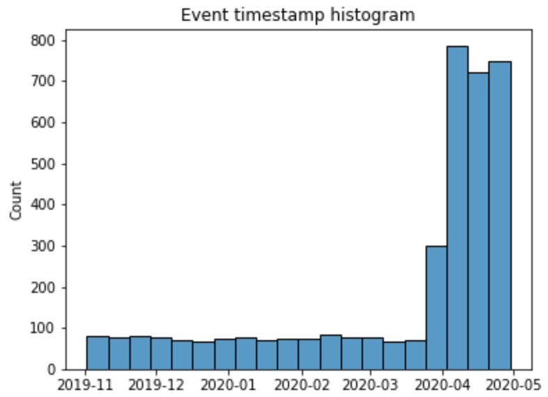
With the Eventstream.event_timestamp_hist() histogram we can notice that the distribution of the new users is not uniform across time: starting from April 2020 the new users number has been surged.
stream2.event_timestamp_hist(event_list=['path_start'])
Let us check whether the new users and the old users have different behavior. First of all, we need to create a segment that will distinguish them. We will consider the new users as those who started their paths after 2020-04-01.
def add_segment_by_date(df):
    first_day = df.groupby('user_id')['timestamp'].min()
    target_index = first_day[first_day < '2020-04-01'].index
    segment_values = df['user_id'].isin(target_index)
    segment_values = segment_values.map({True: 'Before 2020-04', False: 'After 2020-04'})
    return segment_values

stream2 = stream2.add_segment(add_segment_by_date, label='Apr 2020')
Now we can compare the behavior of the new and old users. Let us start from a very basic summary comparing the segment sizes along with a couple of conversion rates: to cart and payment_done events. The Eventstream.segment_overview() method can do this. The definitions of the metrics are similar to the ones in the Eventstream.path_metrics() method. The only difference is that a tuple defining a metric should have 3 elements instead of 2: path metric definition, a function to aggregate the path metric values over a segment, and a metric name. The same string definitions can be used extended with the segment_size literal.
custom_metrics = [
    ('segment_size', 'mean', 'segment size'),
    ('has:cart', 'mean', 'Conversion rate: cart'),
    ('has:payment_done', 'mean', 'Conversion rate: payment_done')
]
stream2.segment_overview('Apr 2020', metrics=custom_metrics)
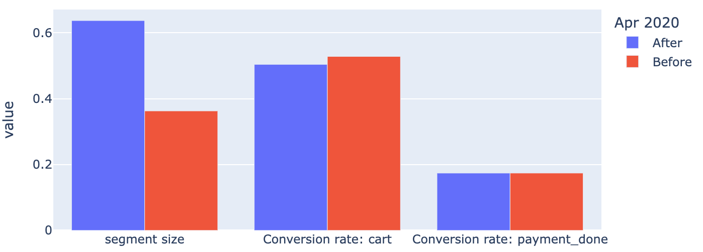
The output shows that from the convertion rates point of view the users are almost identical. The different segment sizes make no sense since the sizes could be of arbitrary values in this case.
The bar chart can be used only if all the metrics are of the same scale. Otherwise it is better to use a heatmap table that can be enabled with the kind='heatmap' argument. Here we use the same metric set extended with the len and time_to: metrics.
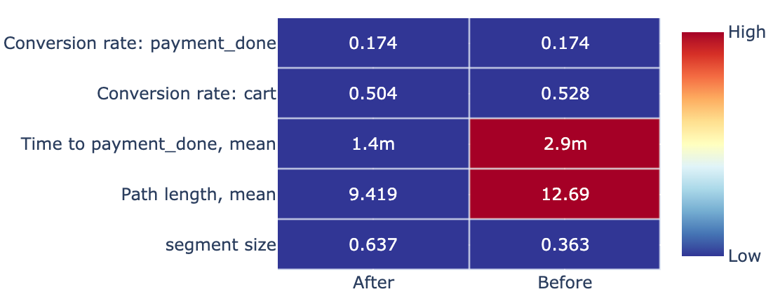
The default axis=1 argument colorize each row separately: the minimum value in each row is deep blue, the maximum value is deep red. axis=0 colorizes the table in column-wise manner. However, for segments of low cardinality the heatmap might be excessive. If we are interested in the numerical values of the table only, we can disable the plot with the show_plot=False argument and access the values property.
stream2.segment_overview(
    segment_name='Apr 2020',
    metrics=custom_metrics,
    kind='heatmap',
    show_plot=False
).values
| Apr 2020 | After | Before |
|---|---|---|
| segment size | 0.637 | 0.363 |
| Path length, mean | 9.419 | 12.69 |
| Time to payment_done, mean | 1.4m | 2.9m |
| Conversion rate: cart | 0.504 | 0.528 |
| Conversion rate: payment_done | 0.174 | 0.174 |
Next, we want to compare the behavior of the new and old users deeper. We will use the step matrix and transition matrix tools for this. Since the segment is binary, when calling these methods we can just pass its name to the groups argument not specifying the segment values.
stream2.step_matrix(groups='Apr 2020', threshold=0)
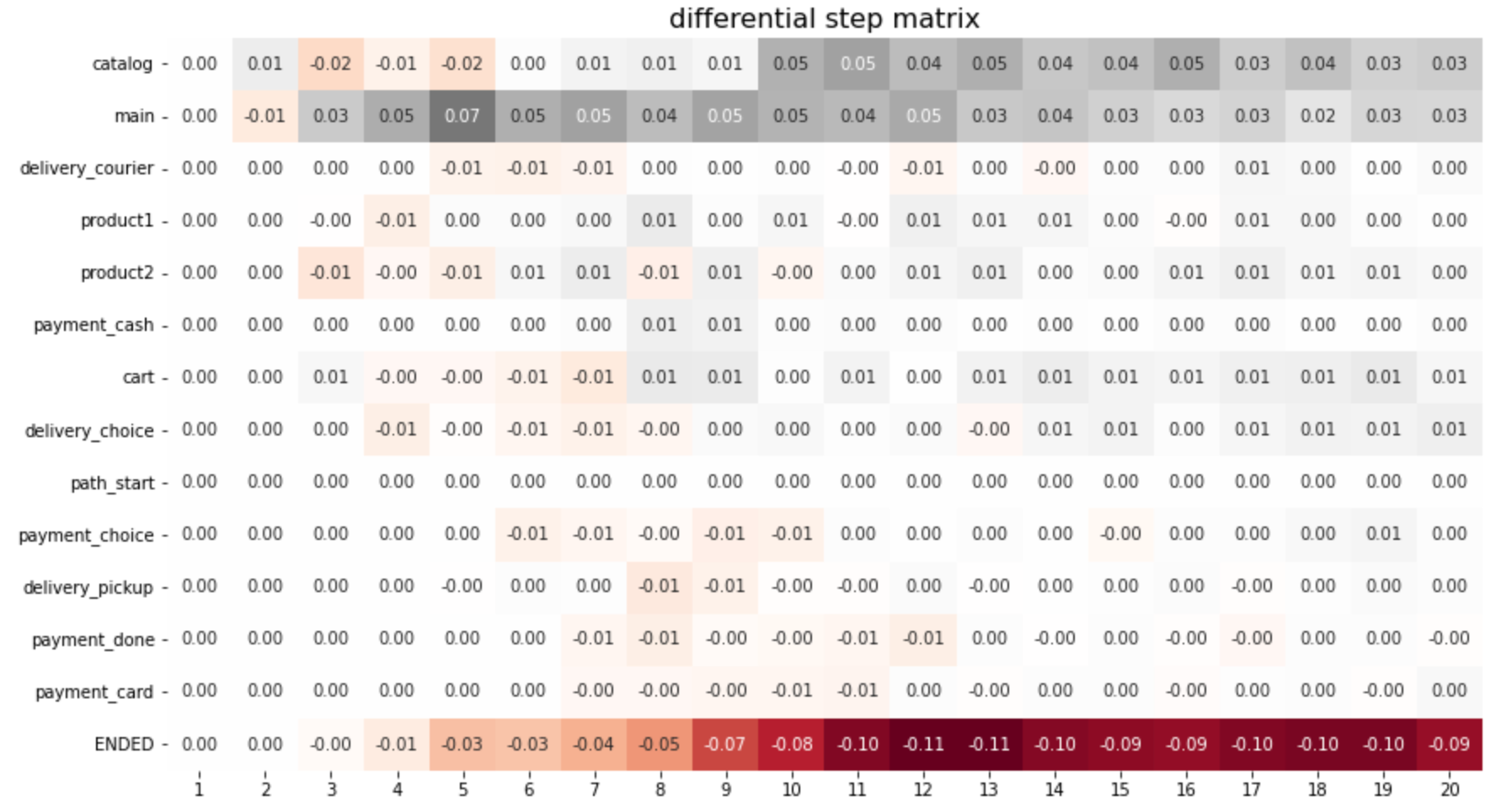
The step matrix reveals that the new users are less likely to surf the catalog and the main page: the grey values in catalog and main rows indicate that the users from Before segment visit these pages more often. Also, the paths of the new users are shorter which is shown by the brown values in the path_end row. But since the conversion rates to cart and payment_done are almost the same, it looks like the new users are more decisive.
stream2.transition_matrix(groups='Apr 2020')
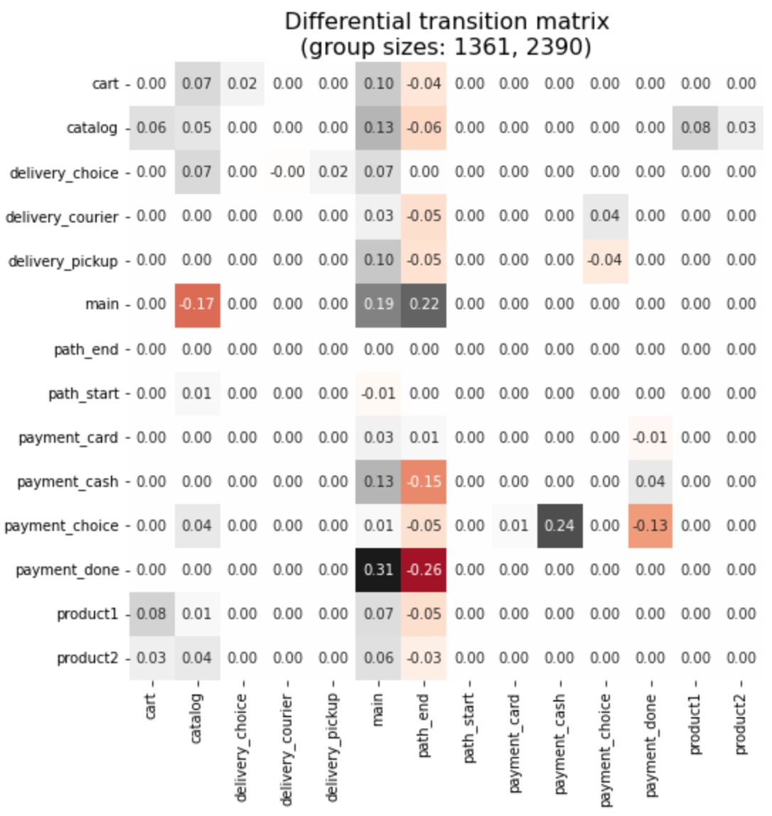
The transitioin matrix exhibits the differences in more detail. The old users tend to transit to the main page from any other page much more often than new users. On the other hand we see many differences in * → path_end transitions. It looks like the old users end up their paths primarily on the main page, while the last event for the new users is distributed more evenly. Finally, we report that the old users prefer cash payment much more than the new users: the difference in payment_choice → payment_cash transition is very high: 0.25.
Clusters#
Retentioneering provides a set of clustering tools that could automatically group users based on their behavior. In a nutshell, the clustering process consists of the following steps:
Path vectorization. Represent the event sequences as a matrix where each row corresponds to a particular path and each column corresponds to a path feature.
Clustering. Apply a clustering algorithm using the feature matrix from the previous step.
Cluster analysis. Analyze the clusters to understand the differences between them.
Vectorization#
First, we calculate the feature set using the Eventstream.extract_features() method. Here we use the simplest configuration: unigrams with the count feature type.
features = stream2.extract_features(ngram_range=(1, 1), feature_type='count')
| main | catalog | ... | cart | payment_done | ||
|---|---|---|---|---|---|---|
| user_id | ||||||
| 122915 | 7 | 18 | ... | 1 | 0 | |
| 463458 | 1 | 8 | ... | 0 | 0 | |
| 1475907 | 2 | 5 | ... | 1 | 0 | |
| 1576626 | 1 | 0 | ... | 0 | 0 | |
| 2112338 | 2 | 3 | ... | 0 | 0 |
Now each path is represented as “bag of unigrams”: a vector of event counts. More feature types such as tfidf, binary, or time-related features are available. See the Eventstream.extract_features() method documentation for more details.
Clustering algorithms#
Next, we apply a clustering algorithm to the feature matrix. The Eventstream.get_clusters() method supports three algorithms: KMeans, HDBSCAN, and GMM. Here we will use KMeans as the most common one. Actually, this algorithm requires the number of clusters to be specified. However, Eventstream.get_clusters() shows the elbow curve plot to help you choose the optimal number of clusters in case you didn’t specify any.
stream2.get_clusters(features, method='kmeans')
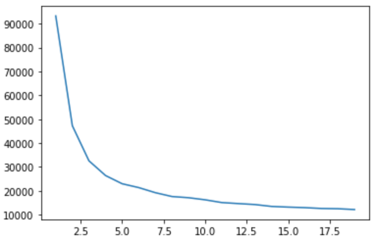
This elbow curve appeared to be too smooth to determine the optimal number of clusters as it often happens in practice. In this case, the number of clusters can be chosen basing on the cluster sizes (they should not be too small). We assume that 8 clusters would be enough and call Eventstream.get_clusters() again with the n_clusters argument set to 8. The cluster partitioning is stored as a regular segment and we can set its name using the segment_name argument.
stream2 = stream2.get_clusters(
    features,
    method='kmeans',
    n_clusters=8,
    random_state=42,
    segment_name='kmeans_clusters'
)
Cluster analysis#
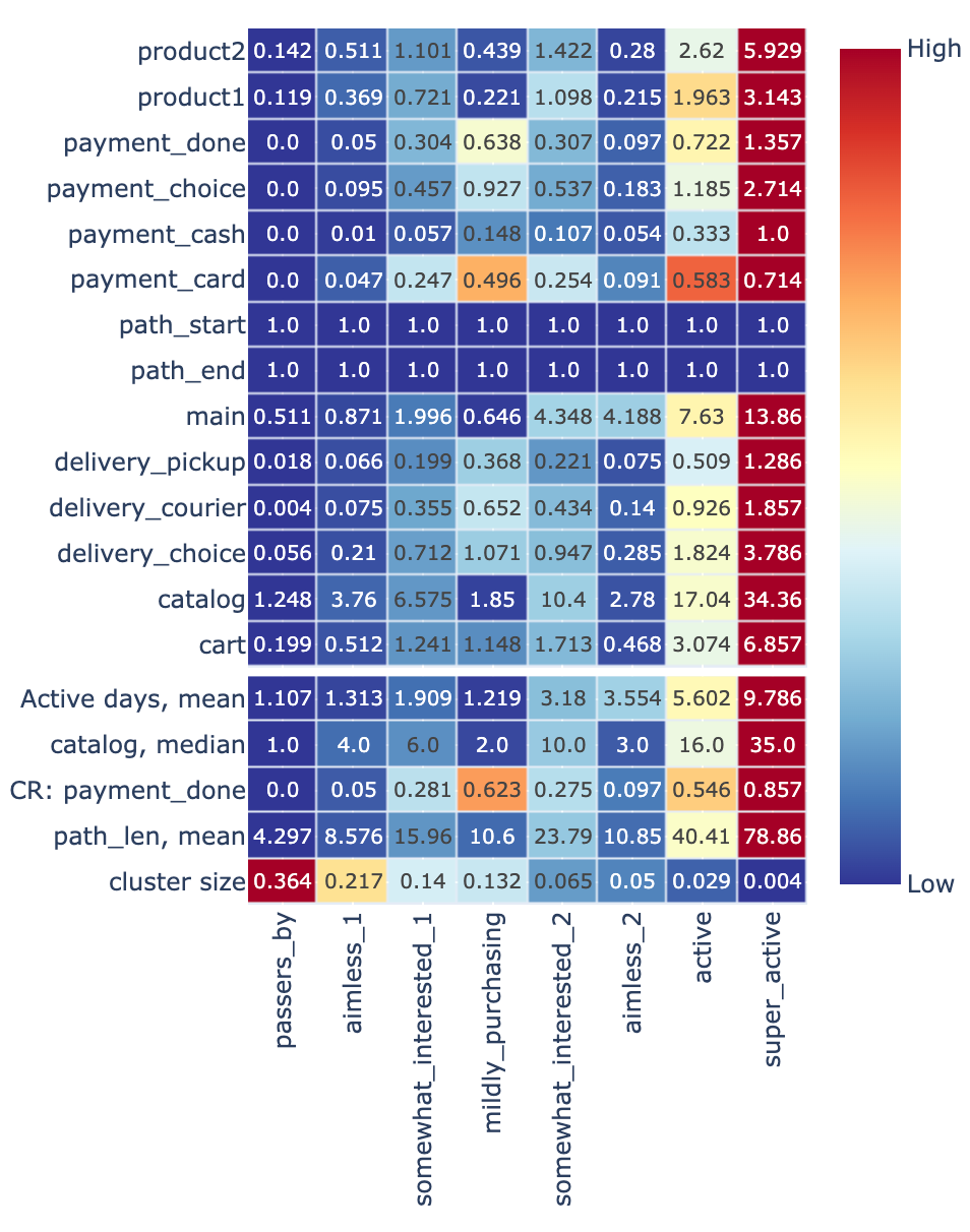
Now kmeans_clusters segment is available for any segment analysis described above. However, since cluster analysis is strongly relate to the feature space that induces the clustering, we can use the Eventstream.clusters_overview() method that better suits this analysis.
stream2.clusters_overview('kmeans_clusters', features, aggfunc='mean', metrics=custom_metrics)
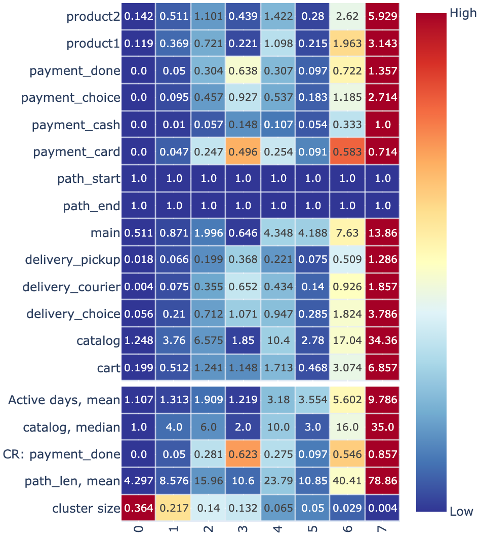
The columns of this table describe the aggregated feature and custom metric values for each cluster. The heatmap (with the default axis=1 parameter) shows how the features values vary across the clusters. For example, the users from the cluster 0 have the lowest activity (all the values in the column 0 are colored in deep blue) while the size of the cluster is the highest (36.4%).
In case we can not see the difference between some clusters clearly looking at the aggregated values only, we can use the Eventstream.segment_diff() method to compare a pair of clusters directly. For example, clusters 2 and 4 look very similar. Let us compare them.
stream2.segment_diff(['kmeans_clusters', '2', '4'], features)
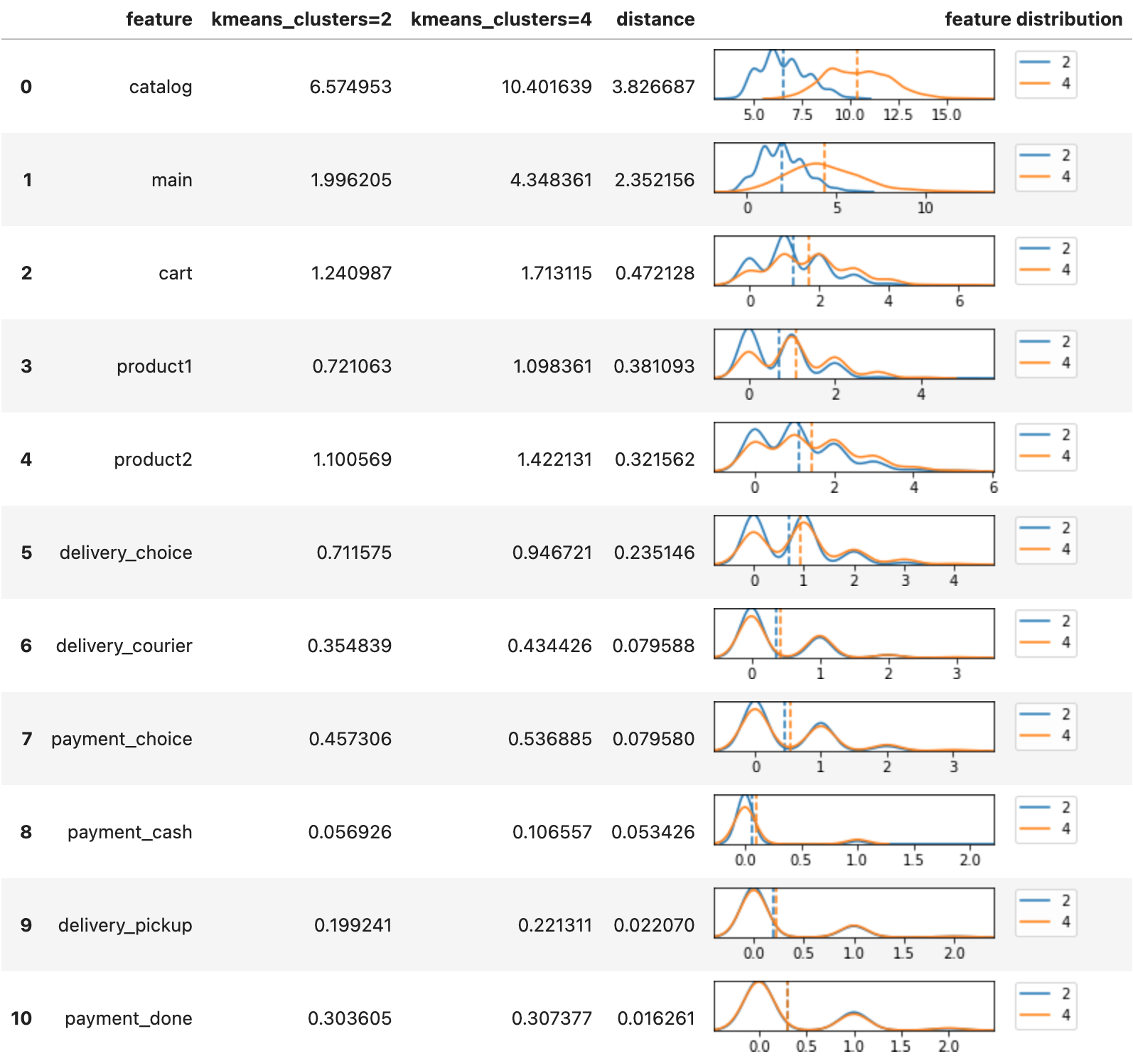
Now we clearly see that the biggest difference between the clusters 2 and 4 is in the catalog and main events distribution.
With a help of the special _OUTER_ literal you can explore the difference of a cluster with the rest of the clusters.
stream2.segment_diff(['kmeans_clusters', '2', '_OUTER_'], features)
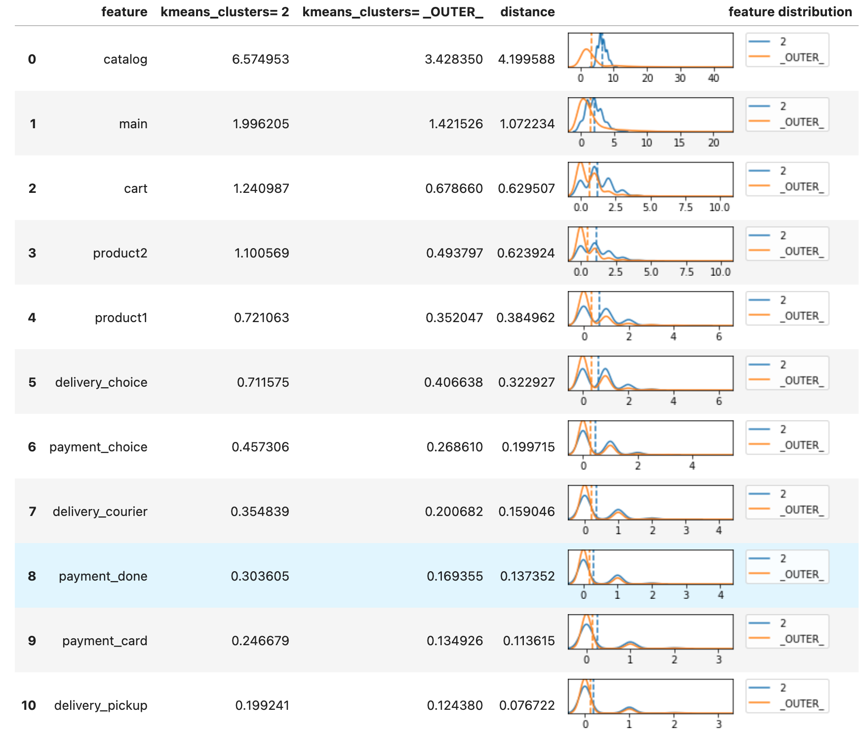
Finally, we can label the clusters with meaningful names using the Eventstream.remap_segment() method and make the same overview visualization for a publication.
cluster_labels = {
    '0': 'passers_by',
    '1': 'aimless_1',
    '2': 'somewhat_interested_1',
    '3': 'mildly_purchasing',
    '4': 'somewhat_interested_2',
    '5': 'aimless_2',
    '6': 'active',
    '7': 'super_active'
}
stream2 = stream2.remap_segment('kmeans_clusters', cluster_labels)
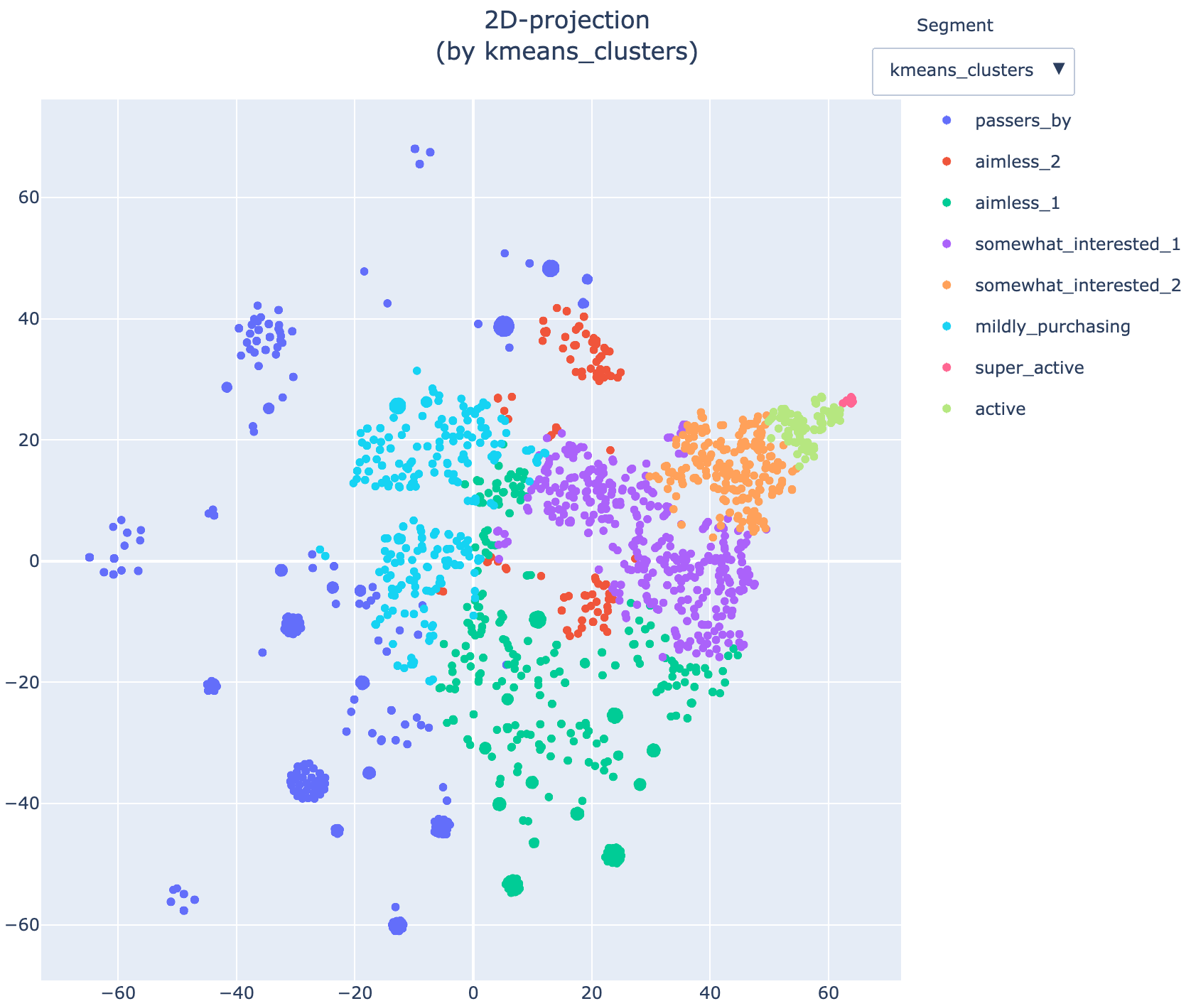
In case we need to get 2D representation of the clusters we can use the Eventstream.projection() method. t-SNE and UMAP algorithms are supported. A fancy dropdown menu allows you to switch between segments. This might be useful when you want to compare multiple clustering versions treating them as different segments. Since the projection is a computationally expensive operation, it is recommended to use the sample_size argument to reduce the number of paths along with the random_state argument to make the results reproducible.
stream2.projection(features=features, sample_size=3000, random_state=42)
