Clusters#
![]()

Loading data#
Throughout this guide we use our demonstration simple_shop dataset. It has already been converted to Eventstream and assigned to stream variable. If you want to use your own dataset, upload it following this instruction.
import numpy as np
import pandas as pd
from retentioneering import datasets

stream = datasets.load_simple_shop()\
    .split_sessions(timeout=(30, 'm'))
Above we use an additional call of the split_sessions data processor helper. We will need this session split in one of the examples in this user guide.
General usage#
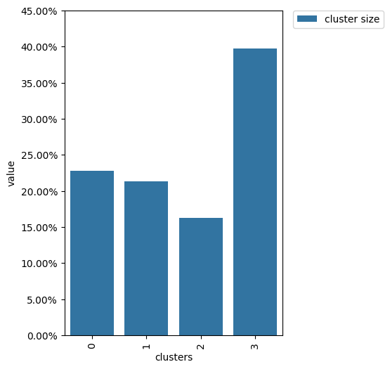
The primary way of using the Clusters tool is sort of traditional. You can create a separate instance of Clusters explicitly, and call extract_features() and fit() methods then. As soon as the clusters are fitted, you can apply multiple tools for cluster analysis. A basic tool that shows cluster sizes and some other statistics is plot().
from retentioneering.tooling.clusters import Clusters

clusters = Clusters(eventstream=stream)
features = clusters.extract_features(feature_type='tfidf', ngram_range=(1, 1))
clusters.fit(method='kmeans', n_clusters=4, X=features, random_state=42)
clusters.plot()

Extracting features#
Before fitting Clusters you need to get features from your data. Clusters.extract_features() is the method that can help with that task. It uses a couple of parameters feature_type and ngram_range, that stands for the type of vectorization. By vectorization we mean the way user trajectories are converted to vectors in some feature space. In general, the vectorization procedure comprises two steps:
Split user paths into short subsequences of particular length called
n-grams.Calculate some statistics taking into account how often each n-gram is represented in a user’s trajectory.
ngram_range argument controls the range of n-gram length to be used in the vectorization. For example, ngram_range=(1, 3) means that we are going to use n-grams of length 1 (single events, that is, unigrams), 2 (bigrams), and 3 (trigrams).
feature type argument stands for the type of vectorization. Besides standard tfidf, count, frequency, and binary features, markov and time-related (time and time_fraction) features are available. See Clusters.extract_features() for the details.
If this vectorization is not enough, you can use your custom features passing it as a pandas DataFrame to the X argument.
Note that if you use the features that are based on n-grams, they are named according to the following pattern event_1 ... event_n_FEATURE_TYPE. For example, for a bigram cart → delivery_choice and feature_type='tfidf', the corresponding feature name will be cart delivery_choice_tfidf.
As for the time-based features such as time, time_fraction, they are associated with a single event, so their names will be cart_time or delivery_choice_time_fraction.
clusters.extract_features(ngram_range=(1, 2), feature_type='tfidf')
| cart_tfidf | cart cart_tfidf | ... | session_start catalog_tfidf | session_start main_tfidf | |
|---|---|---|---|---|---|
| user_id | |||||
| 122915 | 0.049961 | 0.0 | ... | 0.000000 | 0.097361 |
| 463458 | 0.000000 | 0.0 | ... | 0.103926 | 0.000000 |
| ... | ... | ... | ... | ... | ... |
| 999916163 | 0.454257 | 0.0 | ... | 0.181699 | 0.000000 |
| 999941967 | 0.000000 | 0.0 | ... | 0.495717 | 0.000000 |
Fitting clusters#
Fitting clusters is an obligatory step for cluster analysis. If a Clusters object is not fitted (i.e. the clusters are not defined), you can not use any cluster analysis tool. To do this, you can either use pre-defined clustering algorithms such as k-means, or pass custom user-cluster mapping.
Pre-defined clustering methods#
Clusters.fit() is a method for fitting clusters. Its implementation is mainly based on sklearn clustering methods. Here is an example of such a fitting.
clusters = Clusters(eventstream=stream)
features = clusters.extract_features(ngram_range=(1, 2), feature_type='tfidf')
clusters.fit(method='kmeans', n_clusters=4, X=features, random_state=42)
So far the method argument supports two options: kmeans and gmm. n_clusters means the number of clusters since both K-means and GMM algorithms need it to be set. As for the X parameter, it holds features as an input for clusterization algorithms. In our example, the build-in extract_features() method is used to get vectorized features, but the result of custom external vectorization can also be passed. Setting random_state=42 fixes the randomness in the clustering algorithm.
Custom clustering#
You can ignore the pre-defined clustering methods and set custom clusters. To do this, pass user-cluster mapping pandas Series to the Clusters.set_clusters() method. Once the method is called, the Clusters object is considered as fitted, so you can use the cluster analysis methods afterwards.
The following example demonstrates random splitting into 4 clusters. user_clusters variable holds the mapping information on how the users correspond to the clusters. We pass this variable next as an argument for set_clusters method.
import numpy as np

user_ids = stream.to_dataframe()['user_id'].unique()
np.random.seed(42)
cluster_ids = np.random.choice([0, 1, 2, 3], size=len(user_ids))
user_clusters = pd.Series(cluster_ids, index=user_ids)
user_clusters
219483890    2
964964743    3
629881394    0
629881395    2
495985018    2
            ..
125426031    3
26773318     3
965024600    0
831491833    1
962761227    2
Length: 3751, dtype: int64
clusters_random = Clusters(stream)
clusters_random.set_clusters(user_clusters)
clusters_random.plot()
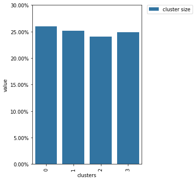
From this diagram, we see that the cluster sizes are close to each other which is exactly what we expect from random splitting.
Cluster analysis methods#
Visualization#
Basic cluster statistics#
The Clusters.plot() method is used for visualizing basic cluster statistics. By default it shows the cluster sizes as the percentage of the eventstream users belonging to a specific cluster. If the targets parameter is defined, the conversion rate for each cluster and each target event is displayed as well. Conversion rate is the proportion of users belonging to a specific cluster who had a target event at least ones.
clusters.plot(targets=['cart', 'payment_done'])
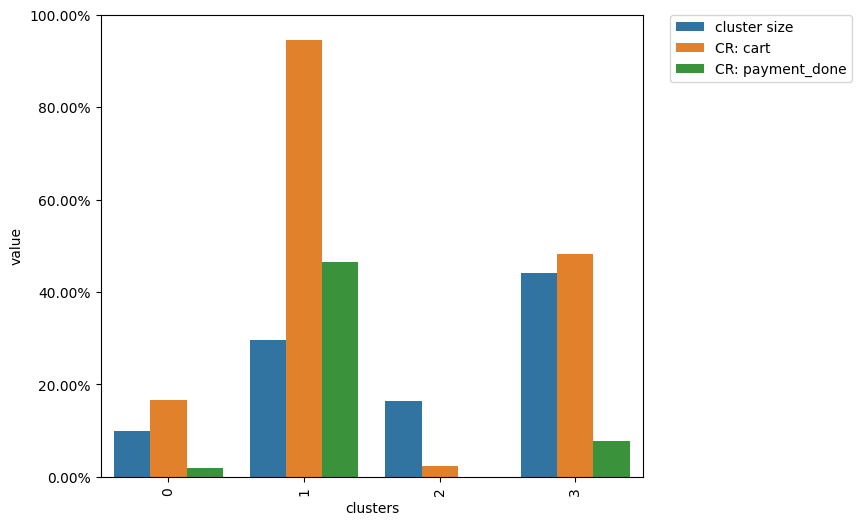
The diagram above shows that cluster 1 contains ~30% of the eventstream users, ~95% of them have at least one cart event in their trajectories, and only ~50% of them successfully paid at least once.
Projections#
Since the feature spaces are of high dimensions, fitted clusters are hard to visualize. For this purpose 2D-projections are used. Due to the nature of projection, it provides a simplified picture, but at least it makes the visualization possible.
Our Clusters.projection() implementation supports two popular and powerful dimensionality reduction techniques: TSNE and UMAP.
clusters.projection(method='tsne')
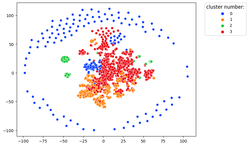
In this image, each dot represents a single user. Users with similar behavior are located close to each other.
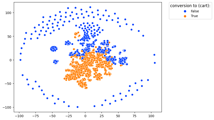
color_type='targets' along with targets argument color the projected dots with respect to conversion rates associated with the events defined in targets. If at least one target event appeared in a user’s trajectory, the user is colored as converted.
clusters.projection(method='tsne', color_type='targets', targets=['cart'])
Exploring individual clusters#
Essentially, any cluster splitting provides nothing but a mapping rule which assigns each user to some group. The way we understand why one cluster differs from another is always tricky. However, either we consider the entire eventstream or its subset (a user cluster), the exploration techniques may be the same. It means having a cluster defined, we can leave the users from this cluster and explore their paths. This is what Clusters.filter_cluster() method is designed for. It returns the narrowed eventstream so we can apply any Retentioneering path analysis tool afterwards. In the following example we apply the transition_graph() method.
clusters\
    .filter_cluster(cluster_id=0)\
    .add_start_end_events()\
    .transition_graph(
        targets={
            'positive': 'payment_done',
            'negative': 'path_end'
        }
    )
Here we additionally used add_start_end_events data processor helper. It adds path_end event that is used as a negative target event in the transition graph.
Clusters comparison#
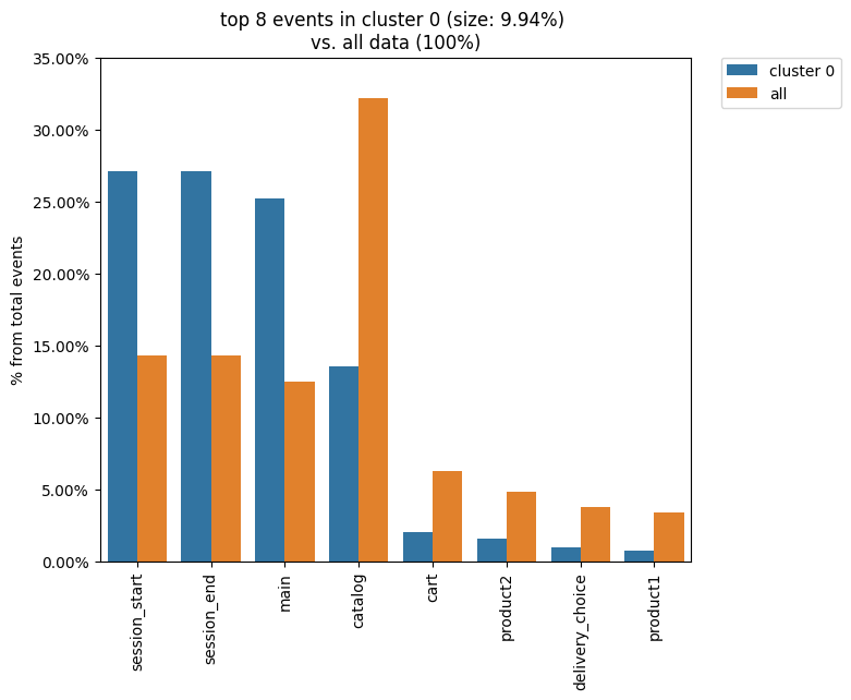
It is natural to describe cluster characteristics in terms of event frequencies generated by the cluster users. Clusters.diff() allows to do this. It takes the cluster_id1 argument as a cluster to be described and plots top_n_events the most frequent events related to this cluster. In comparison, it shows the frequencies of the same events but within the cluster_id2 cluster if the latter is defined. Otherwise, the frequencies over the entire eventstream are shown.
The next example demonstrates that within cluster 0 the main event takes ~27% of all events generated by the users from this cluster, whereas in the original eventstream the main event holds ~13 of all events only.
clusters.diff(cluster_id1=0)
The Clusters tool shares the idea of using weighting column. The most common values for this argument are user_id and session_id (assuming that the session split was created and session_id column exists). If you want to display such cluster statistics as the shares of the unique users or unique sessions, you can use the weight_col argument. Namely, for each event the proportion of the unique user paths/sessions where a particular event appear is calculated.
Also, in the example below we demonstrate the top_n_events argument that controls the number of the events
to be compared.
clusters.diff(cluster_id1=0, top_n_events=5, weight_col='user_id')
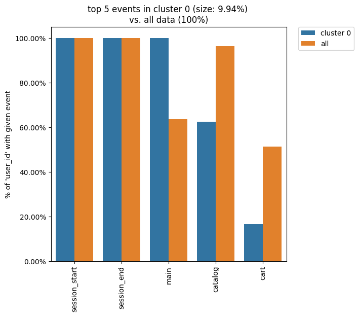
Now, we see that only 60% of the users in cluster 0 had a catalog event, whereas ~97% of the users in the entire eventstream had the same event.
Similarly, by defining weight_col='session_id' we get the following diagram:
clusters.diff(cluster_id1=0, top_n_events=5, weight_col='session_id')
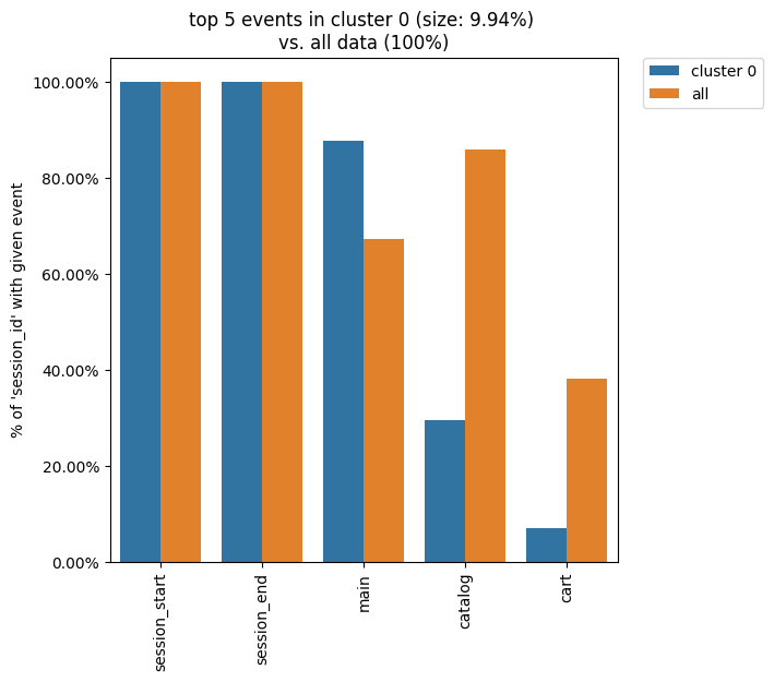
As we see from this diagram, if we look at the sessions generated by the users from cluster 0, only ~30% of these sessions contain at least one catalog event. In comparison, the sessions from the entire eventstream include catalog event in ~84% of cases.
You can not only compare clusters with the whole eventstream, but with other clusters too. Simply define cluster_id2 argument for that.
clusters.diff(cluster_id1=0, cluster_id2=1, top_n_events=5)
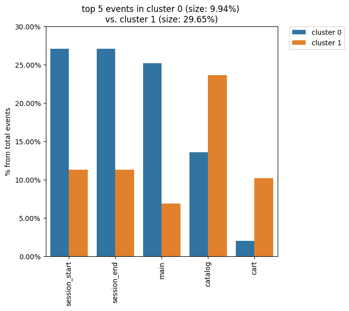
We see that the all bars from the previous diagram have been replaced with the cluster 1 bars.
Note
Some retentioneering tools support groups comparison. For cluster comparison you can also try to use differential step matrix or segmental funnel.
Getting clustering results#
If you want to get the clustering results, there are two methods to do this.
Clusters.user_clusters() returns a pandas.Series containing user_ids as index and cluster_ids as values.
clusters.user_clusters
122915       3
463458       3
1475907      3
1576626      0
2112338      3
            ..
999275109    1
999642905    1
999914554    3
999916163    1
999941967    2
Length: 3751, dtype: int64
Clusters.cluster_mapping()
returns a dictionary containing cluster_id → list of user_ids mapping.
cluster_mapping = clusters.cluster_mapping
list(cluster_mapping.keys())
[0, 1, 2, 3]
Now, we are explicitly confirmed that there are 4 clusters in the result. To get 10 user ids belonging to, say, cluster #0 we can use the following code:
cluster_mapping[0][:10]
[2724645,
 4608042,
 5918715,
 6985523,
 7584012,
 7901023,
 8646372,
 8715027,
 8788425,
 10847418]
Eventstream.clusters property#
There is another way to treat the Clusters tool. This way is aligned with the usage of the most retentioneering tools. Instead of creating an explicit Clusters class instance, you can use Eventstream.clusters property. This property holds a Clusters instance that is embedded right into an eventstream.
clusters = stream.clusters
features = clusters.extract_features(feature_type='tfidf', ngram_range=(1, 1))
clusters.fit(method='kmeans', n_clusters=4, X=features, random_state=42)
clusters.plot()
Note
Once Eventstream.clusters instance is created, it is kept inside the Eventstream object forever until the eventstream is alive. You can re-fit it as many times as you want, but you can not remove it.