Cohorts#
![]()

Cohorts intro#
Cohorts it is a common approach in product analysis that reveals differences and trends in users behavior evolving over time. It helps to indicate the impact of different marketing activities or changes in a product for different time-based groups of users. In particular, cohorts are used to estimate the retention rate of a product users.
The core element of the tool is a cohort matrix. Here is an outline of how it is calculated:
The users are divided into
CohortGroupsdepending on the time of their first appearance in the eventstream. The groups form the rows of the cohort matrix.The timeline is split into
CohortPeriods. They form the columns of the cohort matrix.A value of the cohort matrix is a retention rate of given
CohortGroupsat givenCohortPeriod. Retention rate is the proportion of the users who are still active at given period in comparison with the same users who were active at the first cohort period. We associate user activity with any user event appeared in the eventstream.
To better understand how the cohort tool works, let us consider the following eventstream.
simple_df = pd.DataFrame(
    [
        [1, "event", "2021-01-28 00:01:00"],
        [2, "event", "2021-01-30 00:01:00"],
        [1, "event", "2021-02-03 00:01:00"],
        [3, "event", "2021-02-04 00:01:00"],
        [4, "event", "2021-02-05 00:01:00"],
        [4, "event", "2021-03-06 00:01:00"],
        [1, "event", "2021-03-07 00:01:00"],
        [2, "event", "2021-03-07 00:01:00"],
        [3, "event", "2021-03-29 00:01:00"],
        [5, "event", "2021-03-30 00:01:00"],
        [4, "event", "2021-04-06 00:01:00"]
     ],
     columns=["user_id", "event", "timestamp"]
)
simple_df
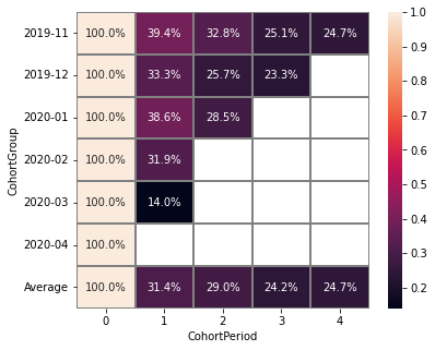
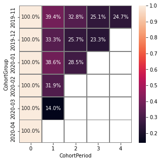
The primary way to build a transition graph is to call Eventstream.cohorts() method. If we split the users into monthly cohorts and check whether they are active on monthly basis, we obtain the following cohort matrix:
from retentioneering.eventstream import Eventstream

simple_stream = Eventstream(simple_df)
simple_stream.cohorts(
    cohort_start_unit='M',
    cohort_period=(1, 'M'),
    average=False
)

CohortGroup- starting datetime of each cohort;CohortPeriod- the number of defined periods from eachCohortGroup.Values- the percentage of active users during a given period.
Each CohortGroup includes users whose acquisition date is within the period from start date of current cohort to the start date of the following cohort (i.e. the first time a user visits your website). So each user belongs to a unique CohortGroup.
Let us take a look at the calculation in details: For the cohort matrix above:
CohortGroupis a month,CohortPeriodis 1 month.
There are 3 CohortGroups in total. Each CohortGroup represents users acquired in a particular month (e.g. the January cohort
(2021-01) includes all users who had their first session in January).
Thus, the values in the column CohortPeriod=0 contain maximum users over each row (Fig. 1), and in the final heatmap it
are always - 100%, users have just joined the eventstream, and no one has left it yet.
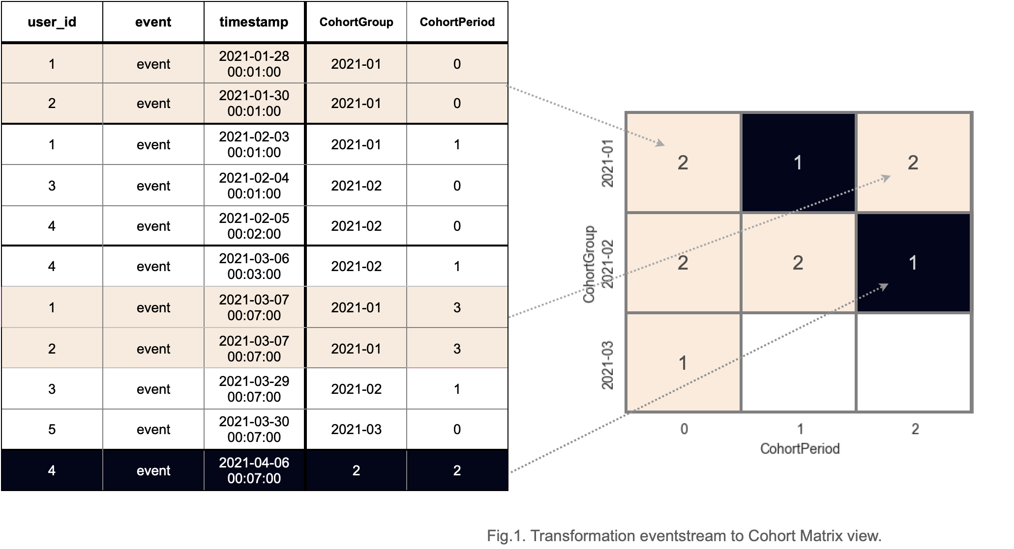
Now let us look at the CohortPeriod=1 . In our case, it is 1 month from the start of the observation period. During the next month, we can see the activity of 50% of users from the first cohort, and 100% of users from the second cohort. The dataset does not cover period 1 of the last cohort (2020-04), so there is no data for this cell, and it remains empty, like all subsequent periods for this cohort.
Finally, CohortPeriod=2. Users 1 and 2 are present in the data for March, so 100% of the users of the first cohort reached the second period. For the second cohort (2021-02) the second period is April, so only user 4 is presented, which means, that only 50% of the users from this cohort reached the second period.
Below we explore how to use and customize the Cohorts tool using retentioneering library. Hereafter we use simple_shop dataset, which has already been converted to Eventstream and assigned to stream variable. If you want to use your own dataset, upload it following this instruction.
from retentioneering import datasets

stream = datasets.load_simple_shop()
Cohort start unit and cohort period#
In the examples we looked at earlier, we used the parameters cohort_start_unit='M' and cohort_period=(1,'M').
stream.cohorts(
    cohort_start_unit='M',
    cohort_period=(1, 'M')
)
The cohort_start_unit parameter is the way of rounding the moment from which the cohort count begins. Minimum timestamp rounding down to the selected datetime unit.
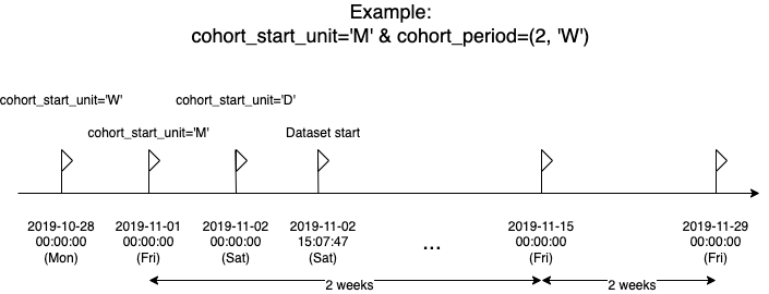
The cohort_period parameter defines time window that you want to examine. It is used for the following:
Start datetime for each
CohortGroup. It means that we take the rounded withcohort_start_unittimestamp of the first click of the first user in the eventstream and count thecohort_periodfrom it. All users who performed actions during this period fall into the first cohort (zero period).CohortPeriodsfor each cohort from its start moment. After the actions described in paragraph 1, we again count the period of the cohort. New users who appeared in the eventstream during this period become the second cohort (zero period). The users from the first cohort who committed actions during this period are counted as the first period of the first cohort.
Let us see what happens when we change the parameters.
stream.cohorts(
    cohort_start_unit='W',
    cohort_period=(3, 'W')
)
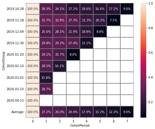
Now, the cohort period lasts 3 weeks, and our heatmap has become more detailed. The number of cohorts also increased from 5 to 8.
Note
Parameters cohort_start_unit and cohort_period should be consistent. Due to “Y” and “M” are non-fixed types it can be used only with each other or if cohort_period_unit is more detailed than cohort_start_unit.
For more details see numpy documentation.
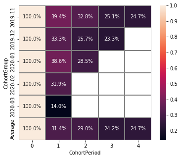
Average values#
If
True- calculating average for each cohort period. Default value.If
False- averages are not calculated.
stream.cohorts(
    cohort_start_unit='M',
    cohort_period=(1, 'M'),
    average=False
)
Cut matrix#
There are three ways to cut the matrix to get rid of boundary values, which can be useful when there is not enough data available at the moment to adequately analyze the behavior of the cohort.
cut_bottom- Drop from cohort_matrix ‘n’ rows from the bottom of the cohort matrix.cut_right- Drop from cohort_matrix ‘n’ columns from the right side.cut_diagonal- Drop from cohort_matrix diagonal with ‘n’ last period-group cells.
Average values are always recalculated.
stream.cohorts(
    cohort_start_unit='M',
    cohort_period=(1, 'M'),
    average=True,
    cut_bottom=1
)
After applying cut_bottom=1, CohortGroup starts from 2020-04 were deleted from our matrix.
stream.cohorts(
    cohort_start_unit='M',
    cohort_period=(1, 'M'),
    average=True,
    cut_bottom=1,
    cut_right=1
)
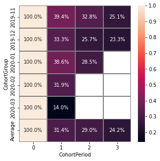
Parameter cut_right allows us to remove the last period column, which reflects information only for the first cohort.
stream.cohorts(
    cohort_start_unit='M',
    cohort_period=(1, 'M'),
    average=True,
    cut_diagonal=1
)
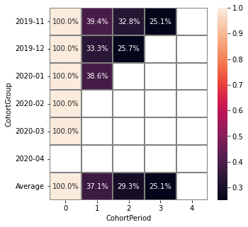
Parameter cut_diagonal deletes values below the diagonal that runs to the left and down from the last period of the first cohort. Thus, we get rid of all boundary values.
Using a separate instance#
By design, Eventstream.cohorts() is a shortcut method that uses Cohorts class under the hood. This method creates an instance of Cohorts class and embeds it into the eventstream object. Eventually, Eventstream.cohorts() returns exactly this instance.
Sometimes it is reasonable to work with a separate instance of Cohorts class. An alternative way to get the same visualization that Eventstream.cohorts() produces is to call Cohorts.fit() and Cohorts.heatmap() methods explicitly. The former method calculates all the values needed for the visualization, the latter displays these values as a heatmap-colored matrix.
from retentioneering.tooling.cohorts import Cohorts

cohorts = Cohorts(eventstream=stream)
cohorts.fit(
    cohort_start_unit='M',
    cohort_period=(1, 'M'),
    average=False
    )
cohorts.heatmap()
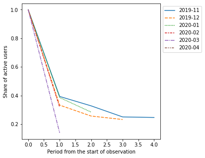
Lineplot#
We can also build lineplots based on our data. By default, each line is one CohortGroup, plot_type='cohorts'.
cohorts.lineplot(width=5, height=5, plot_type='cohorts')
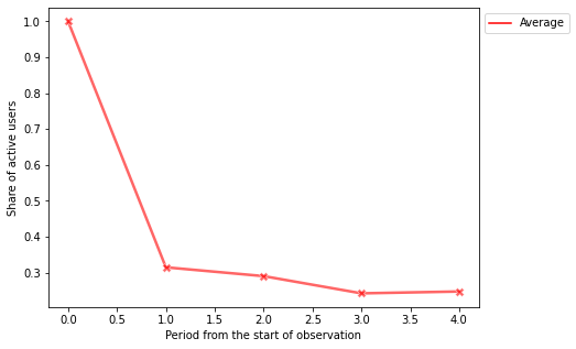
In addition, we can plot the average values for cohorts:
cohorts.lineplot(width=7, height=5, plot_type='average')
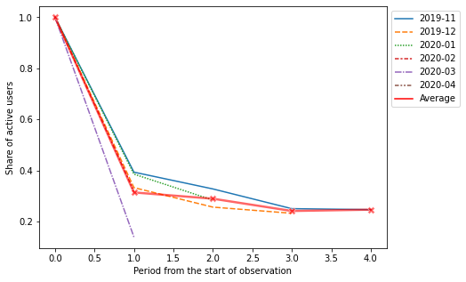
Specifying the plot_type='all' we get a plot that shows lineplot for each cohort and their average values:
cohorts.lineplot(width=7, height=5, plot_type='all');
Common tooling properties#
values#
Cohorts.values property returns the values underlying recent Cohorts.heatmap() call. The property is common for many retentioneering tools. It allows you to avoid unnecessary calculations if the tool object has already been fitted.
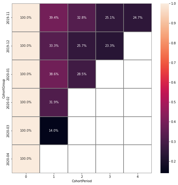
cohorts = stream.cohorts(
    cohort_start_unit='M',
    cohort_period=(1,'M'),
    average=False,
    show_plot=False
).values
| CohortPeriod | 0 | 1 | 2 | 3 | 4 |
|---|---|---|---|---|---|
| CohortGroup | |||||
| 2019-11 | 1.0 | 0.393822 | 0.328185 | 0.250965 | 0.247104 |
| 2019-12 | 1.0 | 0.333333 | 0.257028 | 0.232932 | NaN |
| 2020-01 | 1.0 | 0.386179 | 0.284553 | NaN | NaN |
| 2020-02 | 1.0 | 0.319066 | NaN | NaN | NaN |
| 2020-03 | 1.0 | 0.140000 | NaN | NaN | NaN |
| 2020-04 | 1.0 | NaN | NaN | NaN | NaN |
There are some NANs in the table. These gaps can mean one of two things:
During the specified period, users from the cohort did not perform any actions (and were active again in the next period).
Users from the latest-start cohorts have not yet reached the last periods of the observation. These NaNs are usually concentrated in the lower right corner of the table.
params#
Cohorts.params property returns the Cohorts parameters that was used in the last Cohorts.fit() call.
cohorts.params
{"cohort_start_unit": 'M',
"cohort_period": (1,'M'),
"average": False,
"cut_bottom": 0,
"cut_right": 0,
"cut_diagonal": 0}