Eventstream

What is Eventstream?

Eventstream is the core class in the retentioneering library. This data structure is designed around three following purposes:

• Data container. Eventstream class implements a convenient approach to storing clickstream data.

• Preprocessing. Eventstream allows to efficiently implement a data preparation process. See Preprocessing user guide for more details.

• Applying analytical tools. Eventstream integrates with retentioneering tools and allows you to seamlessly apply them. See user guides on the path analysis tools.

Eventstream creation

Default field names

An Eventstream is a container for clickstream data, that is initialized from a pandas.DataFrame. The class constructor expects the DataFrame to have at least 3 columns: user_id, event, timestamp.

Let us create a dummy DataFrame to illustrate Eventstream init process:

import pandas as pd

df1 = pd.DataFrame(
    [
        ['user_1', 'A', '2023-01-01 00:00:00'],
        ['user_1', 'B', '2023-01-01 00:00:01'],
        ['user_2', 'B', '2023-01-01 00:00:02'],
        ['user_2', 'A', '2023-01-01 00:00:03'],
        ['user_2', 'A', '2023-01-01 00:00:04'],
    ],
    columns=['user_id', 'event', 'timestamp']
)

Having such a dataframe, you can create an eventstream simply as follows:

from retentioneering.eventstream import Eventstream
stream1 = Eventstream(df1)

To do the inverse transformation (i.e. obtain a DataFrame from an eventstream object), to_dataframe() method can be used. However, the method is not just a converter. Using it, we can display the internal Eventstream structure:

stream1.to_dataframe()

	event	timestamp	user_id	event_type	event_index	event_id
0	A	2023-01-01 00:00:00	user_1	raw	0	52c63aed-b1ff-4fea-806d-8484a8978443
1	B	2023-01-01 00:00:01	user_1	raw	1	e9537f88-f776-4047-ae16-66f8b64c4076
2	B	2023-01-01 00:00:02	user_2	raw	2	bb6f1cd3-a630-4d48-94c2-8a3cf5a3d22f
3	A	2023-01-01 00:00:03	user_2	raw	3	3680e70b-166d-475d-8ac1-166ea213f5f4
4	A	2023-01-01 00:00:04	user_2	raw	4	c22d97a7-63a1-4d57-b738-16863107dfb7

We will describe the columns of the resulting DataFrame later in Displaying eventstream section.

Changing default field names

For custom DataFrame column names you can either rename them using pandas, or set a mapping rule that would tell the Eventstream constructor the mapping to the correct column names. This can be done with Eventstream attribute raw_data_schema with uses RawDataSchema class under the hood.

Let us illustrate its usage with the following example with the same dataframe containing the same data but with different column names (client_id, action and datetime):

df2 = pd.DataFrame(
    [
        ['user_1', 'A', '2023-01-01 00:00:00'],
        ['user_1', 'B', '2023-01-01 00:00:01'],
        ['user_2', 'B', '2023-01-01 00:00:02'],
        ['user_2', 'A', '2023-01-01 00:00:03'],
        ['user_2', 'A', '2023-01-01 00:00:04']
    ],
     columns=['client_id', 'action', 'datetime']
)

raw_data_schema = {
    'user_id': 'client_id',
    'event_name': 'action',
    'event_timestamp': 'datetime'
}

stream2 = Eventstream(df2, raw_data_schema=raw_data_schema)
stream2.to_dataframe().head(3)

	event	timestamp	user_id	event_type	event_index	event_id
0	A	2023-01-01 00:00:00	user_1	raw	0	0fd741dd-8140-4182-8046-cf23906208c6
1	B	2023-01-01 00:00:01	user_1	raw	1	3a4db2d7-a4b8-4845-ab21-0950f6a2bfc0
2	B	2023-01-01 00:00:02	user_2	raw	2	fd4552d9-db28-47cc-b7a1-4408a895cff9

As we see, raw_data_schema argument maps fields client_id, action, and datetime so that they are imported to the eventstream correctly.

Custom columns

Another common case is when your DataFrame has some additional columns that you want to add to the eventstream. By default, these columns are included automatically. In case you want to explicitly control what columns should be included, you can add them in the custom_cols argument.

Suppose the initial DataFrame now also contains two columns: session and device, and you want to leave the former column only. Then you can use custom_cols parameter that works as a whitelist.

df3 = pd.DataFrame(
    [
        ['user_1', 'A', '2023-01-01 00:00:00', 'session_1', 'mobile'],
        ['user_1', 'B', '2023-01-01 00:00:01', 'session_1', 'mobile'],
        ['user_2', 'B', '2023-01-01 00:00:02', 'session_2', 'desktop'],
        ['user_2', 'A', '2023-01-01 00:00:03', 'session_3', 'desktop'],
        ['user_2', 'A', '2023-01-01 00:00:04', 'session_3', 'desktop']
    ],
    columns=['client_id', 'action', 'datetime', 'session', 'device']
)

raw_data_schema = {
    'user_id': 'client_id',
    'event_name': 'action',
    'event_timestamp': 'datetime',
}

stream3 = Eventstream(df3, raw_data_schema=raw_data_schema, custom_cols=['session'])
stream3.to_dataframe().head(3)

	event	timestamp	user_id	event_type	session	event_index	event_id
0	A	2023-01-01 00:00:00	user_1	raw	session_1	0	c15ff01a-6822-464f-a4cc-dc6118e44e6d
1	B	2023-01-01 00:00:01	user_1	raw	session_1	1	359c5e0e-d533-4101-8f9c-86247cb78590
2	B	2023-01-01 00:00:02	user_2	raw	session_2	2	ce03482c-0b47-42eb-9947-8ee3cc39ecd9

As we see from above, the session column was included in the eventstream while device was not.

The same results could be achieved if you pass custom_cols as a key in the RawDataSchema. In this case, the value must be a list of dictionaries, one dict per one custom field. A single dict must contain two fields: raw_data_col and custom_col. The former stands for a field name from the sourcing dataframe, the latter stands for the corresponding field name to be set in the resulting eventstream.

raw_data_schema = {
    'user_id': 'client_id',
    'event_name': 'action',
    'event_timestamp': 'datetime',
    'custom_cols': [
        {
            'raw_data_col': 'session',
            'custom_col': 'session_id'
        }
    ]
}

stream3 = Eventstream(df3, raw_data_schema=raw_data_schema)
stream3.to_dataframe().head(3)

Here we see that the original session column is stored in session_id column, according to the defined raw_data_schema

If the core triple columns of the DataFrame are titled with the default names user_id, event, timestamp (instead of client_id, action, datetime) then you can ignore their mapping in the raw_data_schema and pass custom_cols argument only.

Eventstream field names

You can also set the names of the eventstream columns (the default names are user_id, event, timestamp) by defining schema argument. It is a dictionary with the following possible keys, the values are the desired column names. In the example below we set a schema for the same stream1 and define the names of the basic columns as client_id, action, and datetime:

new_eventstream_schema = {
    'user_id': 'client_id',
    'event_name': 'action',
    'event_timestamp': 'datetime'
}

stream1_new_schema = Eventstream(df1, schema=new_eventstream_schema)
stream1_new_schema.to_dataframe().head(3)

	action	datetime	client_id	event_type	event_index	event_id
0	A	2023-01-01 00:00:00	user_1	raw	0	884a38f1-dc62-4567-a10b-5c20a690a173
1	B	2023-01-01 00:00:01	user_1	raw	1	8ed1d3fb-8026-413a-a426-9f8858cd9d73
2	B	2023-01-01 00:00:02	user_2	raw	2	965de90a-6a68-42a5-8d8a-8e23534bfd72

The full list of an eventstream fields and the corresponding values is available in Eventstream.schema attribute:

stream1_new_schema.schema

EventstreamSchema(
    event_id='event_id',
    event_type='event_type',
    event_index='event_index',
    event_name='action',
    event_timestamp='datetime',
    user_id='client_id',
    custom_cols=[]
)

Path start and end

For many practical reasons it is useful to keep synthetic events indicating path start and path end. Eventstream constructor adds path_start and path_end events explicitly. See also add_start_end_events data processor.

User sampling

Contemporary data analysis usually involve working with large datasets. Using retentioneering to work with such datasets might cause the following undesirable effects:

• High computational costs.

• The messy big picture (especially in case of applying such tools as Transition Graph, StepMatrix and StepSankey). Insufficient user paths or large number of almost identical paths (especially short paths) often add no value to the analysis. It might be reasonable to get rid of them.

• Due to Eventstream design, all the data uploaded to an Eventstream instance is kept immutable. Even if you remove some eventstream rows while preprocessing, the data stays untouched: it just becomes hidden and is marked as removed. Thus, the only chance to tailor the dataset to a reasonable size is to sample the user paths at entry point - while applying Eventstream constructor.

The size of the original dataset can be reduced by path sampling. In theory, this procedure could affect the eventstream analysis, especially in case you have rare but important events and behavioral patterns. Nevertheless, the sampling is less likely to distort the big picture, so we recommend to use it when it is needed.

We also highlight that user path sampling means that we remove some random paths entirely. We guarantee that the sampled paths contain all the events from the original dataset, and they are not truncated.

There are a couple sampling parameters in the Eventstream constructor: user_sample_size and user_sample_seed. There are two ways of setting the sample size:

• A float number. For example, user_sample_size=0.1 means that we want to leave 10% ot the paths and remove 90% of them.

• An integer sample size is also possible. In this case a specified number of events will be left.

user_sample_seed is a standard way to make random sampling reproducible (see this Stack Overflow explanation). You can set it to any integer number.

Below is a sampling example for simple_shop dataset.

from retentioneering import datasets

simple_shop_df = datasets.load_simple_shop(as_dataframe=True)
sampled_stream = Eventstream(
    simple_shop_df,
    user_sample_size=0.1,
    user_sample_seed=42
)

print('Original number of the events:', len(simple_shop_df))
print('Sampled number of the events:', len(sampled_stream.to_dataframe()))

unique_users_original = simple_shop_df['user_id'].nunique()
unique_users_sampled = sampled_stream.to_dataframe()['user_id'].nunique()

print('Original unique users number: ', unique_users_original)
print('Sampled unique users number: ', unique_users_sampled)

Original number of the events: 32283
Sampled number of the events: 3298
Original unique users number:  3751
Sampled unique users number:  375

We see that the number of the users has been reduced from 3751 to 375 (10% exactly). The number of the events has been reduced from 32283 to 3298 (10.2%), but we didn’t expect to see exact 10% here.

Displaying eventstream

Now let us look at columns represented in an eventstream and discuss to_dataframe() method using the example of stream3 eventstream.

stream3.to_dataframe()

	event	timestamp	user_id	session_id	event_type	event_index	event_id
0	A	2023-01-01 00:00:00	user_1	session_1	raw	0	7427d9f5-8666-4821-b0a9-f74a962f6d72
1	B	2023-01-01 00:00:01	user_1	session_1	raw	1	6c9fef69-a176-45d1-bb13-628796e68602
2	B	2023-01-01 00:00:02	user_2	session_2	raw	2	7aee8104-b1cc-4df4-8a8d-f569395ffad9
3	A	2023-01-01 00:00:03	user_2	session_3	raw	3	3b3610b2-8016-4259-bf68-6daf34518e34
4	A	2023-01-01 00:00:04	user_2	session_3	raw	4	945e6514-2f41-457c-ba70-2ac35150b41e

Besides the standard triple user_id, event, timestamp and custom column session_id we see the columns event_id, event_type, event_index. These are some technical columns, containing the following:

• event_type - all the events that come from the sourcing DataFrame are of raw event type. However, preprocessing methods can add some synthetic events that have various event types. See the details in data processors user guide.

• event_index - an integer which is associated with the event order. By default, an eventstream is sorted by timestamp, and optionally by event column. As for the synthetic events which are often placed at the beginning or in the end of a user’s path, special sorting is applied. See explanation of index and reindex logic for the details and also data processors user guide. Please note that the event index might has duplicated values. It is ok due to its design.

• event_id - a string identifier of an eventstream row.

There are additional arguments that may be useful.

• show_deleted. Eventstream is immutable data container. It means that all the events once uploaded to an eventstream are kept. Even if we remove some events, they are just marked as removed. By default, show_deleted=False so these events are hidden in the output DataFrame. If show_deleted=True, all the events from the original state of the eventstream and all the in-between preprocessing states are displayed.

• copy - when this flag is True (by default it is False) then an explicit copy of the DataFrame is created. See details in pandas documentation.

Eventstream index and reindex

In the previous section, we have already mentioned the sorting algorithm when we described special event_type and event_index eventstream columns. Now, let us take a closer look at the sorting logic and illustrate it with several examples.

By default, raw events are sorted by timestamp column. So the events with the same timestamps are kept in the same order as they are represented in the sourcing DataFrame. In case you need some custom ordering for the events with the same timestamps use the events_order parameter. For example, due to some technical reasons events can arrive at the server with the same timestamp and randomly change the order and create unnecessary variability.

After initial sorting, the relative order of raw events is fixed, and re-sorting is not possible.

In the dummy dataframe below, there are two users, each with a pair of events (“A” and “B”) that have equal timestamps. If we create an eventstream with default parameters, the order will be preserved, exactly the same as in the input dataframe.

df4 = pd.DataFrame(
    [
        ['user_1', 'A', '2023-01-01 00:00:00'],
        ['user_1', 'B', '2023-01-01 00:00:00'],
        ['user_2', 'B', '2023-01-01 00:00:03'],
        ['user_2', 'A', '2023-01-01 00:00:03'],
        ['user_2', 'A', '2023-01-01 00:00:04']
    ],
    columns=['user_id', 'event', 'timestamp']
)

stream4 = Eventstream(df4)
stream4.to_dataframe()

	event	timestamp	user_id	event_type	event_index
0	A	2023-01-01 00:00:00	user_1	raw	0
1	B	2023-01-01 00:00:00	user_1	raw	1
2	B	2023-01-01 00:00:03	user_2	raw	2
3	A	2023-01-01 00:00:03	user_2	raw	3
4	A	2023-01-01 00:00:04	user_2	raw	4

Now we create a new Eventstream from our dummy DataFrame, but with the specified events_order=["B", "A"] parameter. As we can see, the first two events have swapped places.

Eventstream(df4, events_order=["B", "A"]).to_dataframe()

	event	timestamp	user_id	event_type	event_index
0	B	2023-01-01 00:00:00	user_1	raw	0
1	A	2023-01-01 00:00:00	user_1	raw	1
2	B	2023-01-01 00:00:03	user_2	raw	2
3	A	2023-01-01 00:00:03	user_2	raw	3
4	A	2023-01-01 00:00:04	user_2	raw	4

As for the synthetic events which are often placed at the beginning or in the end of a user’s path, special sorting is applied. There is a set of pre-defined event types, that are arranged in the following default order:

IndexOrder = [
    "profile",
    "path_start",
    "new_user",
    "existing_user",
    "cropped_left",
    "session_start",
    "session_start_cropped",
    "group_alias",
    "raw",
    "raw_sleep",
    None,
    "synthetic",
    "synthetic_sleep",
    "positive_target",
    "negative_target",
    "session_end_cropped",
    "session_end",
    "session_sleep",
    "cropped_right",
    "absent_user",
    "lost_user",
    "path_end"
]

Most of these types are created by build-in data processors. Note that some of the types are not used right now and were created for future development.

To see full explanation about which data processor creates which event_type you can explore the data processors user guide.

If needed, you can pass a custom sorting list to the Eventstream constructor as the index_order argument.

In case you already have an eventstream instance, you can assign a custom sorting list to Eventstream.index_order attribute. Afterwards, you should use index_events() method to apply this new sorting. For demonstration purposes we use here a AddPositiveEvents data processor, which adds new event with prefix positive_target_.

add_events_stream = stream4.add_positive_events(targets=['B'])
add_events_stream.to_dataframe()

	event	timestamp	user_id	event_type	event_index
0	A	2023-01-01 00:00:00	user_1	raw	0
1	B	2023-01-01 00:00:00	user_1	raw	1
2	positive_target_B	2023-01-01 00:00:00	user_1	positive_target	1
3	B	2023-01-01 00:00:03	user_2	raw	2
4	positive_target_B	2023-01-01 00:00:03	user_2	positive_target	2
5	A	2023-01-01 00:00:03	user_2	raw	3
6	A	2023-01-01 00:00:04	user_2	raw	4

We see that positive_target_B events with type positive_target follow their raw parent event B. Assume we would like to change their order.

custom_sorting = [
    'profile',
    'path_start',
    'new_user',
    'existing_user',
    'cropped_left',
    'session_start',
    'session_start_cropped',
    'group_alias',
    'positive_target',
    'raw',
    'raw_sleep',
    None,
    'synthetic',
    'synthetic_sleep',
    'negative_target',
    'session_end_cropped',
    'session_end',
    'session_sleep',
    'cropped_right',
    'absent_user',
    'lost_user',
    'path_end'
]

add_events_stream.index_order = custom_sorting
add_events_stream.index_events()
add_events_stream.to_dataframe()

	event	timestamp	user_id	event_type	event_index
0	A	2023-01-01 00:00:00	user_1	raw	0
1	positive_target_B	2023-01-01 00:00:00	user_1	positive_target	1
2	B	2023-01-01 00:00:00	user_1	raw	1
3	positive_target_B	2023-01-01 00:00:03	user_2	positive_target	2
4	B	2023-01-01 00:00:03	user_2	raw	2
5	A	2023-01-01 00:00:03	user_2	raw	3
6	A	2023-01-01 00:00:04	user_2	raw	4

As we can see, the order of the events changed, and now raw events B follow positive_target_B events.

Descriptive methods

Eventstream provides a set of methods for a first touch data exploration. To showcase how these methods work, we need a larger dataset, so we will use our simple_shop dataset. For demonstration purposes, we add session_id column by applying SplitSessions data processor.

from retentioneering import datasets

stream_with_sessions = datasets\
    .load_simple_shop()\
    .split_sessions(timeout=(30, 'm'))

stream_with_sessions.to_dataframe().head()

	event	timestamp	user_id	session_id	event_type	event_index	event_id
0	session_start	2019-11-01 17:59:13.273932	219483890	219483890_1	session_start	0	92aa043e-02ac-4a4d-9f37-4bfc9dd101dc
1	catalog	2019-11-01 17:59:13.273932	219483890	219483890_1	raw	1	c1368d21-85fe-4ed0-864b-87b79eca8076
3	product1	2019-11-01 17:59:28.459271	219483890	219483890_1	raw	3	4f437751-b117-4ef2-ba23-e91fe3a022fc
5	cart	2019-11-01 17:59:29.502214	219483890	219483890_1	raw	5	740eeca9-db1f-4279-a0aa-ceb07de60638
7	catalog	2019-11-01 17:59:32.557029	219483890	219483890_1	raw	7	4f0d2ba7-396f-492e-bbf0-887ef14211e6

General statistics

Describe

In a similar fashion to pandas, we use describe() for getting a general description of an eventstream.

stream_with_sessions.describe()

		value
category	metric
overall	unique_users	3751
	unique_events	14
	unique_sessions	6454
	eventstream_start	2019-11-01 17:59:13
	eventstream_end	2020-04-29 12:48:07
	eventstream_length	179 days 18:48:53
path_length_time	mean	9 days 11:15:18
	std	23 days 02:52:25
	median	0 days 00:01:21
	min	0 days 00:00:00
	max	149 days 04:51:05
path_length_steps	mean	12.05
	std	11.43
	median	9.0
	min	3
	max	122
session_length_time	mean	0 days 00:00:52
	std	0 days 00:01:08
	median	0 days 00:00:30
	min	0 days 00:00:00
	max	0 days 00:23:44
session_length_steps	mean	7.0
	std	4.18
	median	6.0
	min	3
	max	55

The output consists of three main categories:

• overall statistics

• full user-path statistics

  • time distribution

  • steps (events) distribution

• sessions statistics

  • time distribution

  • steps (events) distribution

session_col parameter is optional and points to the eventstream column that contains session ids (session_id is the default value). If such a column is defined, session statistics are also included. Otherwise, the values related to sessions are not displayed.

There is one more parameter - raw_events_only (default False) that could be useful if some synthetic events have already been added by adding data processors. Note that those events affect all “*_steps” categories.

Now let us go through the main categories and take a closer look at some of the metrics:

overall

By eventstream start and eventstream end in the “Overall” block we denote timestamps of the first event and the last event in the eventstream correspondingly. eventstream_length is the time distance between event stream start and end.

path/session length time and path/session length steps

These two blocks show some time-based statistics over user paths and sessions. Categories “path/session_length_time” and “path/session length steps” provide similar information on the length of users paths and sessions correspondingly. The former is calculated in days and the latter in the number of events.

It is important to mention that all the values in “*_steps” categories are rounded to the 2nd decimal digit, and in “*_time” categories - to seconds. This is also true for the next method.

Describe events

The describe_events() method provides event-wise statistics about an eventstream. Its output consists of three main blocks:

1. basic statistics

2. full user-path statistics,

   • time to first occurrence (FO) of each event,

   • steps to first occurrence (FO) of each event,

3. sessions statistics (if this column exists),

   • time to first occurrence (FO) of each event,

   • steps to first occurrence (FO) of each event.

You can find detailed explanations of each metric in api documentation.

The default parameters are session_col='session_id', raw_events_only=False. With them, we will get statistics for each event present in our data. These two arguments work exactly the same way as in the describe() method.

stream = datasets.load_simple_shop()
stream.describe_events()

	basic_statistics				time_to_FO_user_wise					steps_to_FO_user_wise
	number_of_occurrences	unique_users	number_of_occurrences_shared	unique_users_shared	mean	std	median	min	max	mean	std	median	min	max
event
cart	2842	1924	0.09	0.51	3 days 08:59:14	11 days 19:28:46	0 days 00:00:56	0 days 00:00:01	118 days 16:11:36	4.51	4.09	3.0	1	41
catalog	14518	3611	0.45	0.96	0 days 05:44:21	3 days 03:22:32	0 days 00:00:00	0 days 00:00:00	100 days 08:19:51	0.30	0.57	0.0	0	7
delivery_choice	1686	1356	0.05	0.36	5 days 09:18:08	15 days 03:19:15	0 days 00:01:12	0 days 00:00:03	118 days 16:11:37	6.78	5.56	5.0	2	49
delivery_courier	834	748	0.03	0.20	6 days 18:14:55	16 days 17:51:39	0 days 00:01:28	0 days 00:00:06	118 days 16:11:38	8.96	6.84	7.0	3	45
delivery_pickup	506	469	0.02	0.13	7 days 21:12:17	18 days 22:51:54	0 days 00:01:34	0 days 00:00:06	114 days 01:24:06	9.51	8.06	7.0	3	71
main	5635	2385	0.17	0.64	3 days 20:15:36	9 days 02:58:23	0 days 00:00:07	0 days 00:00:00	97 days 21:24:23	2.00	2.94	1.0	0	20
payment_card	565	521	0.02	0.14	6 days 21:42:26	17 days 18:52:33	0 days 00:01:40	0 days 00:00:08	138 days 04:51:25	11.14	7.34	9.0	5	65
payment_cash	197	190	0.01	0.05	13 days 23:17:25	24 days 00:00:02	0 days 00:02:18	0 days 00:00:10	118 days 16:11:39	14.15	11.10	9.5	5	73
payment_choice	1107	958	0.03	0.26	6 days 12:49:38	17 days 02:54:51	0 days 00:01:24	0 days 00:00:06	118 days 16:11:39	9.42	6.37	7.0	4	52
payment_done	706	653	0.02	0.17	7 days 01:37:54	17 days 09:10:00	0 days 00:01:34	0 days 00:00:08	115 days 09:18:59	12.21	8.29	10.0	5	84
product1	1515	1122	0.05	0.30	5 days 23:49:43	16 days 04:36:13	0 days 00:00:50	0 days 00:00:00	118 days 19:38:40	5.46	6.04	3.0	1	61
product2	2172	1430	0.07	0.38	4 days 06:13:24	13 days 03:26:17	0 days 00:00:34	0 days 00:00:00	126 days 23:36:45	4.32	4.51	3.0	1	36

If the number of unique events in an eventstream is high, we can leave events only from the list defined in event_list parameter. In the example below we leave the cart and payment_done events only as the events of high importance. We also transpose the output DataFrame for a nicer view.

stream.describe_events()
stream.describe_events(event_list=['payment_done', 'cart']).T

	event	cart	payment_done
basic_statistics	number_of_occurrences	2842	706
	unique_users	1924	653
	number_of_occurrences_shared	0.09	0.02
	unique_users_shared	0.51	0.17
time_to_FO_user_wise	mean	3 days 08:59:14	7 days 01:37:54
	std	11 days 19:28:46	17 days 09:10:00
	median	0 days 00:00:56	0 days 00:01:34
	min	0 days 00:00:01	0 days 00:00:08
	max	118 days 16:11:36	115 days 09:18:59
steps_to_FO_user_wise	mean	4.51	12.21
	std	4.09	8.29
	median	3.0	10.0
	min	1	5
	max	41	84

Often, such simple descriptive statistics are not enough to deeply understand the time-related values, so we want to see their distribution. For these purposes the following group of methods has been implemented.

Time-based histograms

User lifetime

One of the most important time-related statistics is user lifetime. By lifetime we mean the time distance between the first and the last event represented in a user’s trajectory. The histogram for this variable is plotted by user_lifetime_hist() method.

stream.user_lifetime_hist()

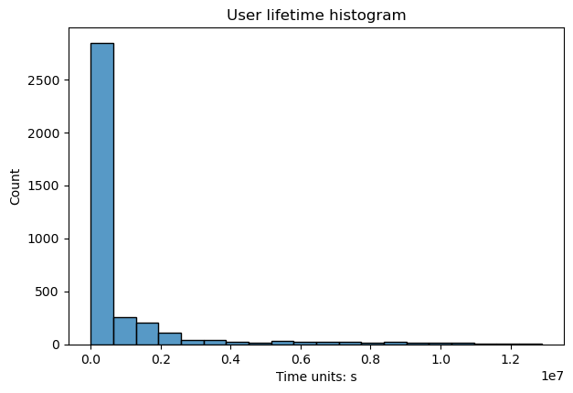
The method has multiple parameters:

• timedelta_unit defines a datetime unit that is used for the lifetime measuring;

• log_scale sets logarithmic scale for the bins;

• lower_cutoff_quantile, upper_cutoff_quantile indicate the lower and upper quantiles (as floats between 0 and 1), the values between the quantiles only are considered for the histogram;

• bins defines the number of histogram bins. Also can be the name of a reference rule or number of bins. See details in numpy documentation;

• width and height set figure width and height in inches.

Note

The method is especially useful for selecting parameters to DropPaths. See the user guide on preprocessing for details.

Timedelta between two events

Previously, we have defined user lifetime as the timedelta between the beginning and the end of a user’s path. This can be generalized. timedelta_hist() method shows a histogram for the distribution of timedeltas between a couple of specified events.

The method supports similar formatting arguments (timedelta_unit, log_scale, lower_cutoff_quantile, upper_cutoff_quantile, bins, width, height) as we have already mentioned in user_lifetime_hist method.

If no arguments are passed (except formatting arguments), timedeltas between all adjacent events are calculated within each user path. For example, this tiny eventstream

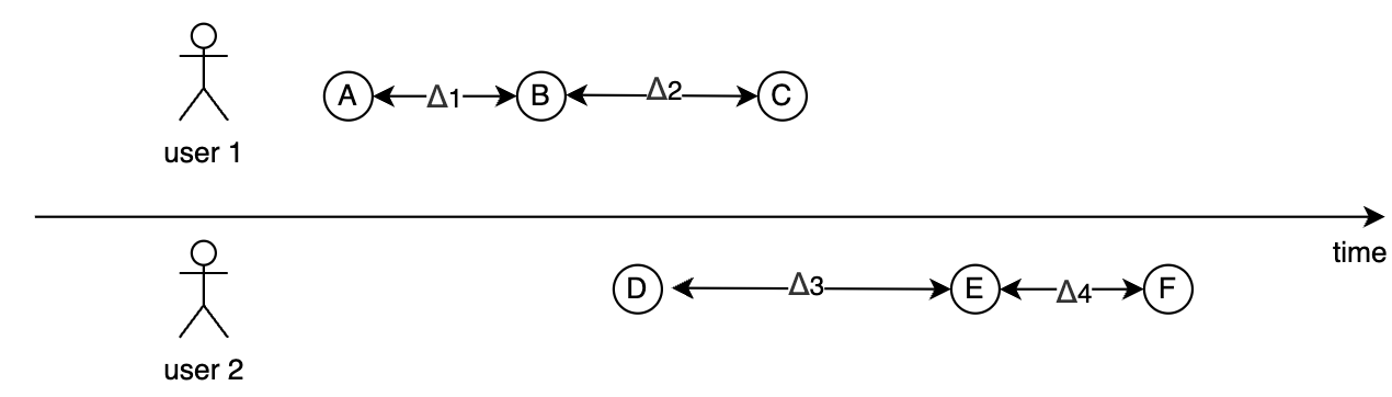
generates 4 timedeltas \(\Delta_1, \Delta_2, \Delta_3, \Delta_4\) as shown in the diagram. The timedeltas between events B and D, D and C, C and E are not taken into account because two events from each pair belong to different users.

Here is how the histogram looks for the simple_shop dataset with log_scale=True and timedelta_unit='m':

stream.timedelta_hist(log_scale=True, timedelta_unit='m')

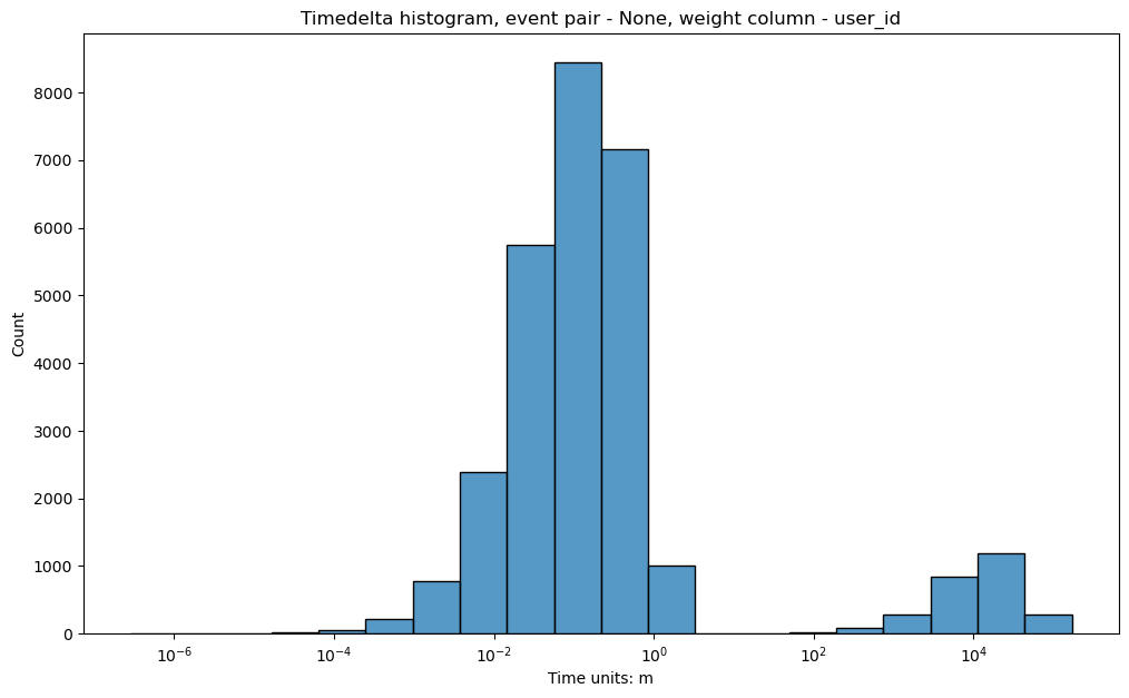
This distribution of the adjacent events fairly common. It looks like a bimodal (which is not true: remember we use log-scale here), but these two bells help us to estimate a timeout for splitting sessions. From this charts we can see that it is reasonable to set it to some value between 10 and 100 minutes.

Be careful if there are some synthetic events in the data. Usually those events are assigned with the same timestamp as their “parent” raw events. Thus, the distribution of the timedeltas between events will be heavily skewed to 0. Parameter raw_events_only=True can help in such a situation. Let us add to our dataset some common synthetic events using AddStartEndEvents and SplitSessions data processors.

stream_with_synthetic = datasets\
    .load_simple_shop()\
    .add_start_end_events()\
    .split_sessions(timeout=(30, 'm'))

stream_with_synthetic.timedelta_hist(log_scale=True, timedelta_unit='m')
stream_with_synthetic.timedelta_hist(
    raw_events_only=True,
    log_scale=True,
    timedelta_unit='m'
)

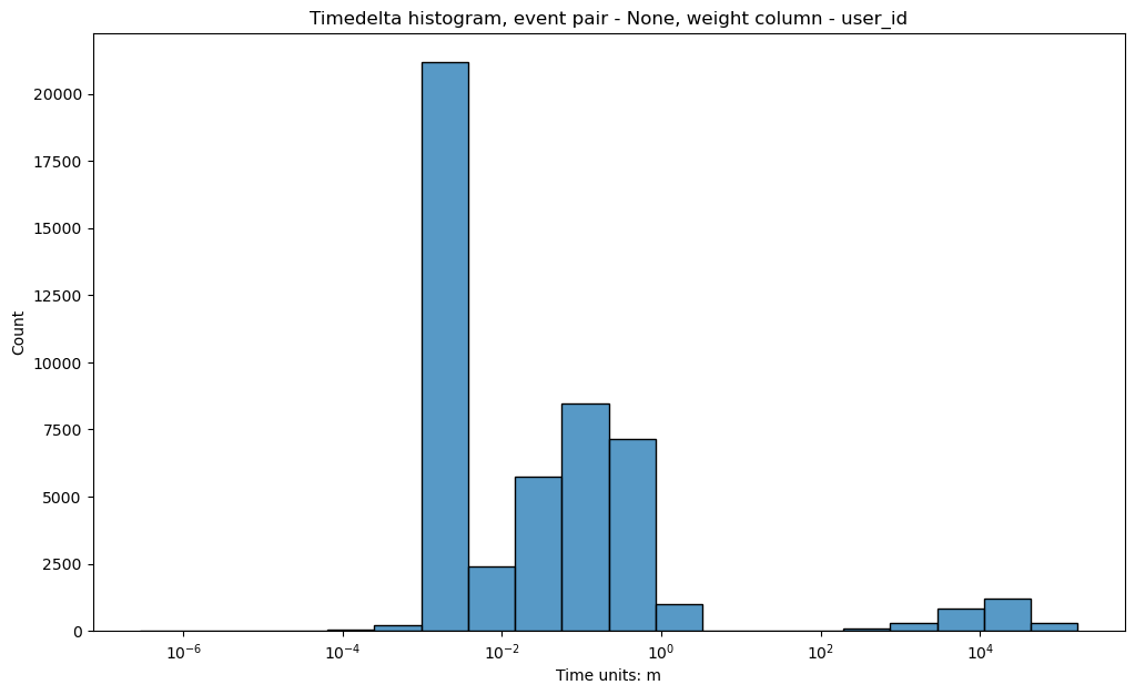
You can see that on the second plot there is no high histogram bar located at \(\approx 10^{-3}\), so that the second histogram looks more natural.

Another use case for timedelta_hist() is visualizing the distribution of timedeltas between two specific events. Assume we want to know how much time it takes for a user to go from product1 to cart. Then we set event_pair=('product1', 'cart') and pass it to timedelta_hist:

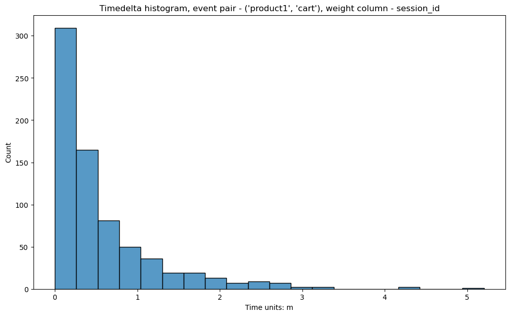
stream.timedelta_hist(event_pair=('product1', 'cart'), timedelta_unit='m')

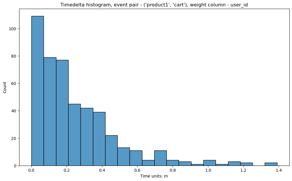
From the Y scale, we see that such occurrences are not very numerous. This is because the method still works with only adjacent pairs of events (in this case product1 and cart are assumed to go one right after another in a user’s path). That is why the histogram is skewed to 0. adjacent_events_only parameter allows us to work with any cases when a user goes from product1 to cart non-directly but passing through some other events:

stream.timedelta_hist(
    event_pair=('product1', 'cart'),
    timedelta_unit='m',
    adjacent_events_only=False
)

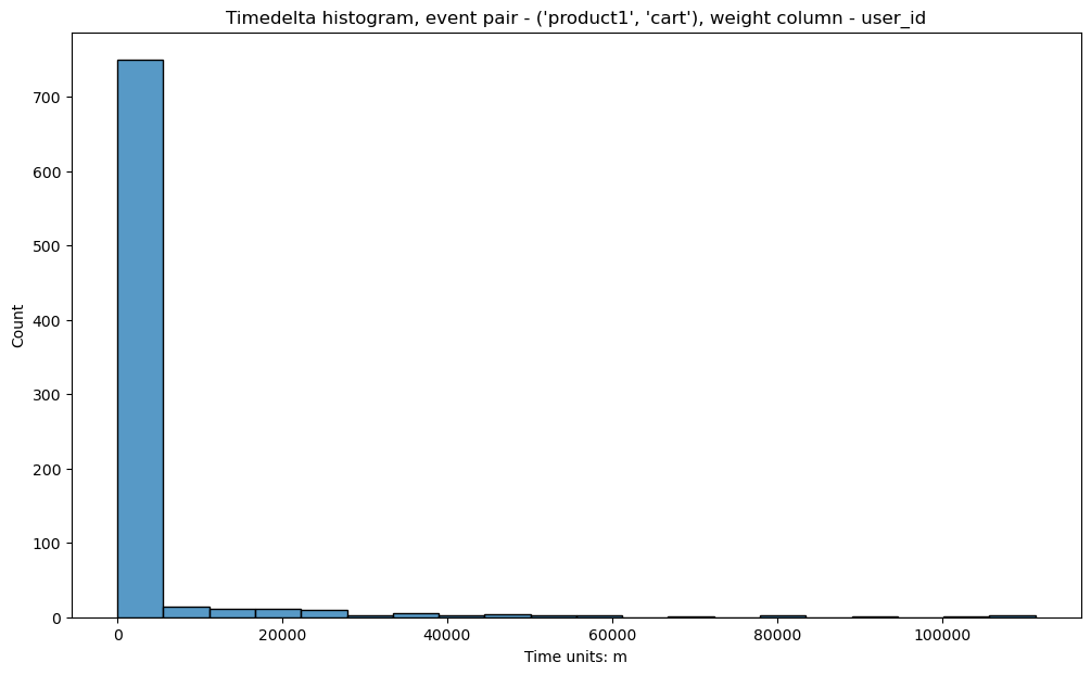
We see that the number of observations has increased, especially around 0. In other words, for the vast majority of the users transition product1 → cart takes less than 1 day. On the other hands, we observe a “long tail” of the users whose journey from product1 to cart takes multiple days. We can interpret this as there are two behavioral clusters: the users who are open for purchases, and the users who are picky. However, we also notice that adding a product to a cart does not necessarily mean that a user intends to make a purchase. Sometimes users adds an item to a cart just to check its final price, delivery options, etc.

Here we should make a stop and explain how timedeltas between event pairs are calculated. Below you can see the picture of one user path and timedeltas that will be displayed in a timedelta_hist with the parameters event_pair=('A', 'B') and adjacent_events_only=False.

Let us consider each time delta calculation:

• \(\Delta_1\) is calculated between ‘A’ and ‘B’ events. ‘D’ and ‘F’ are ignored because of adjacent_events_only=False.

• The next ‘A’ event is colored grey and is skipped because there is one more ‘A’ event closer to the ‘B’ event. In such cases, we pick the ‘A’ event, that is closer to the next ‘B’ and calculate \(\Delta_2\).

Single user path

Now let us get back to our example. Due to the fact we have a lot of users with short trajectories and a few users with very long paths our histogram is unreadable.

To make entire plot more comprehensible - the log_scale parameter can be used. We have already used that parameter for the x axis, but it is also available fot the y axis. For example: log_scale=(False, True).

Another way to resolve that problem, is to look separately on different parts of our plot. For that purpose we can use parameters lower_cutoff_quantile and upper_cutoff_quantile. These parameters specify boundaries for the histogram and will be applied last.

In the example below, firstly, we keep users with event_pair=('product1', 'cart') and adjacent_events_only=False, and after it we truncate 90% of users with the shortest trajectories and keep 10% of the longest.

stream.timedelta_hist(
        event_pair=('product1', 'cart'),
        timedelta_unit='m',
        adjacent_events_only=False,
        lower_cutoff_quantile=0.9
    )

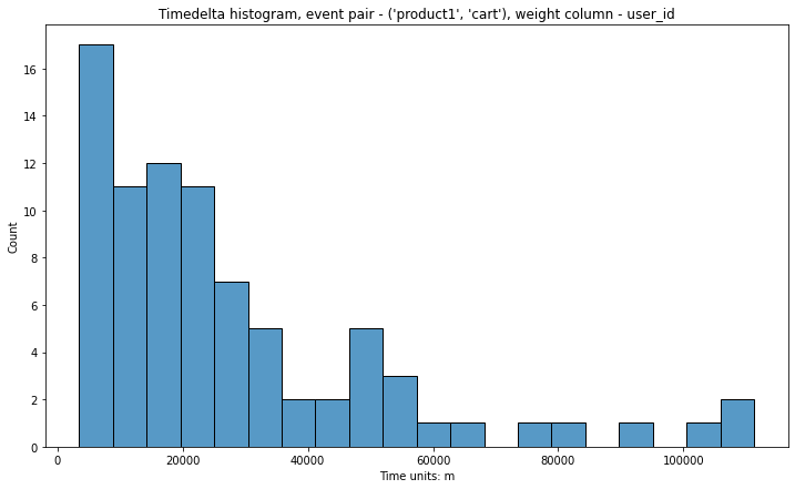
Here it is the same algorithm, but 10% of users with the shortest trajectories will be kept.

stream.timedelta_hist(
        event_pair=('product1', 'cart'),
        timedelta_unit='m',
        adjacent_events_only=False,
        upper_cutoff_quantile=0.1
    )

If we set both parameters, boundaries will be calculated simultaneously and truncated afterward.

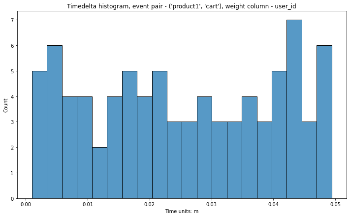
Let us turn to another case. Sometimes we are interested in looking only at events within a user session. If we have already split the paths into sessions, we can use weight_col='session_id':

stream_with_synthetic\
    .timedelta_hist(
        event_pair=('product1', 'cart'),
        timedelta_unit='m',
        adjacent_events_only=False,
        weight_col='session_id'
    )

It is clear now that within a session the users walk from product1 to cart event in less than 3 minutes.

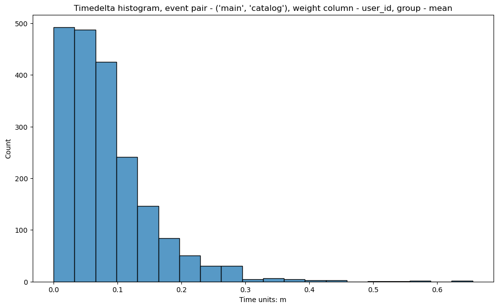
For frequently occurring events we might be interested in aggregating the timedeltas over sessions or users. For example, transition main -> catalog is quite frequent. Some users do these transitions quickly, some of them do not. It might be reasonable to aggregate the timedeltas over each user path first (we would get one value per one user at this step), and then visualize the distribution of these aggregated values. This can be done by passing an additional argument time_agg='mean' or time_agg='median'.

stream\
    .timedelta_hist(
        event_pair=('main', 'catalog'),
        timedelta_unit='m',
        adjacent_events_only=False,
        weight_col='user_id',
        time_agg='mean'
    )

Eventstream global events

event_pair argument can accept a couple of auxiliary events: eventstream_start and eventstream_end. They indicate the first and the last events in an evenstream.

It is especially useful for choosing left_cutoff and right_cutoff parameters for LabelCroppedPaths data processor. Before you choose it, you can explore how a path’s beginning/end margin from the right/left edge of an eventstream. In the histogram below, \(\Delta_1\) illustrates such a margin for event_pair=('eventstream_start', 'B'). Note that here only one timedelta is calculated - from the ‘eventstream_start’ to the first occurrence of specified event.

\(\Delta_1\) in the following example illustrates a margin for event_pair=('B', 'eventstream_end'). And again, only one timedelta per userpath is calculated - from the ‘B’ event (its last occurrence) to the ‘eventstream_end’.

stream_with_synthetic\
    .timedelta_hist(
        event_pair=('eventstream_start', 'path_end'),
        timedelta_unit='h',
        adjacent_events_only=False
    )

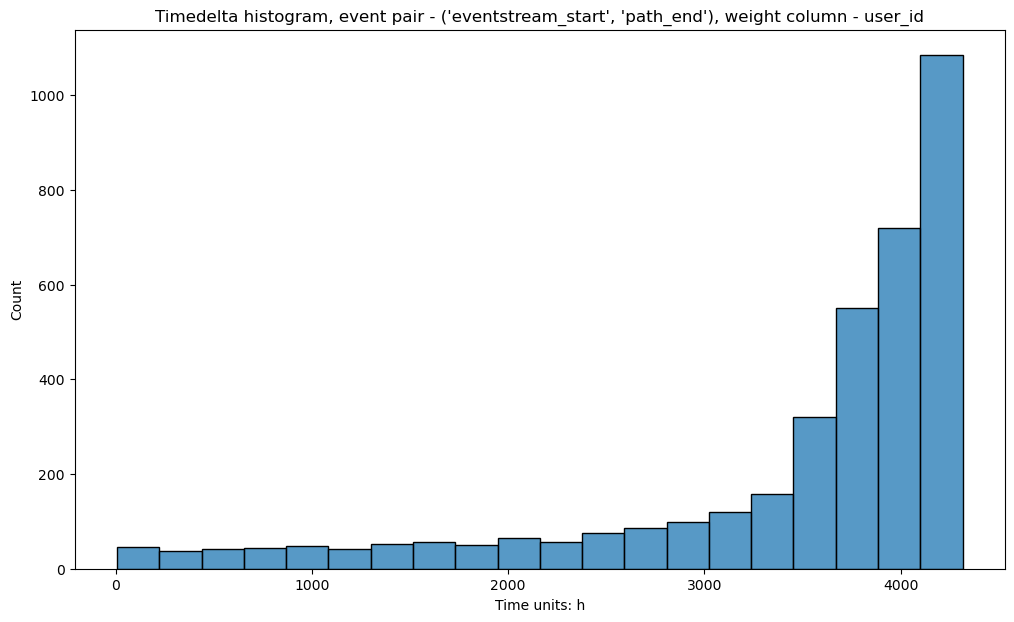
For more details on how this histogram helps to define left_cutoff and right_cutoff parameters see LabelCroppedPaths section in the data processors user guide.

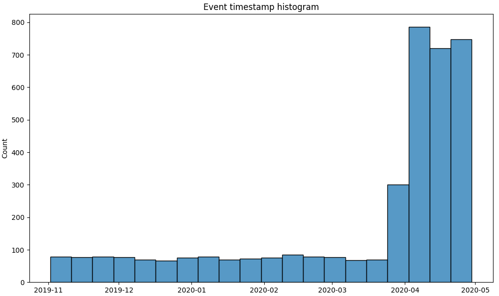
Event intensity

There is another helpful diagram that can be used for eventstream overview. Sometimes we want to know how the events are distributed over time. The histogram for this distribution is plotted by event_timestamp_hist() method.

stream.event_timestamp_hist()

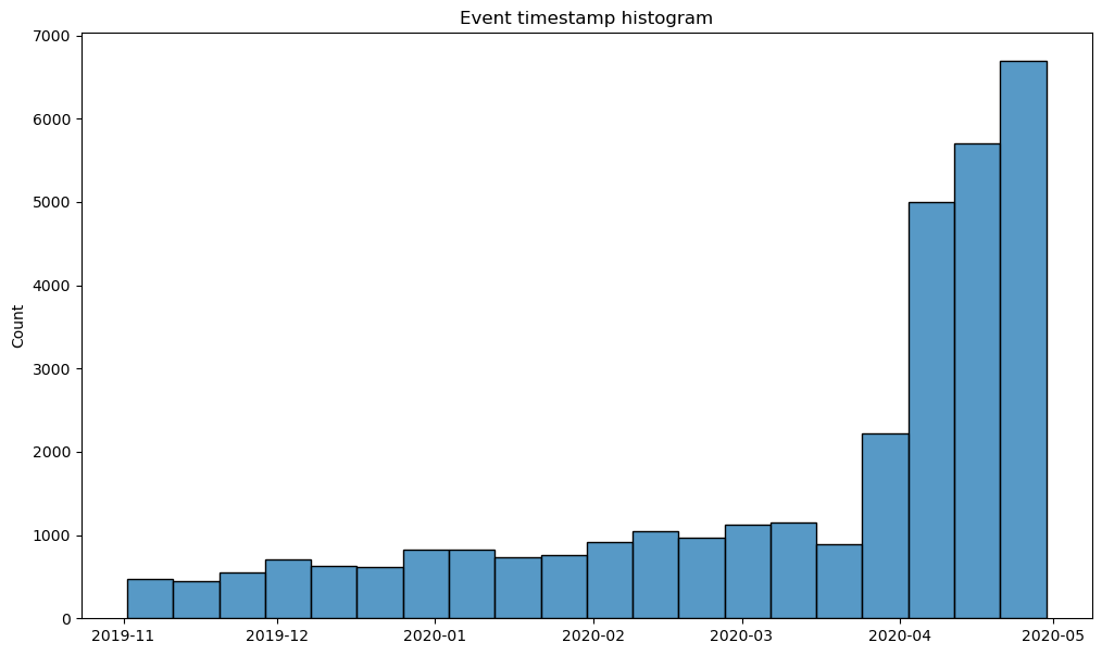
We can notice the heavy skew in the data towards the period between April and May of 2020. One of the possible interpretations of this fact is that the product worked in beta version until April 2020, and afterwards a stable were released so that new users started to arrive much more intense. event_timestamp_hist has event_list argument, so we can check this hypothesis by choosing path_start in the event list .

stream\
    .add_start_end_events()\
    .event_timestamp_hist(event_list=['path_start'])

From this histogram we see that our hypothesis is true. New users started to arrive much more intense in April 2020.

Similar to timedelta_hist(), event_timestamp_hist also has parameters raw_events_only, upper_cutoff_quantile, lower_cutoff_quantile, bins, width and height that work with the same logic.